Welch’s Analysis of Variance (ANOVA)

Author

Christofer Rodriguez & Said Salehe

Published

June 6, 2023

Introduction

Welch’s one-way Analysis of Variance (ANOVA) tests for equal means in a one-way design (not assuming equal variance). This is is an alternative to the standard one-way ANOVA in the situation where the homogeneity of variance assumption is violated.

You should run Welch’s test in all cases where you have normally distributed data that violates the assumption of homogeneity of variance.

Packages

Code

library(rstatix)
library(gt)
library(skimr)
library(jmv)
library(tidyverse)

Data Download

Data used in this example can be downloaded Here.(Frost 2023) There was no data dictionary available for this data set, however, the data was described as “the ground reaction forces that are generated by jumping from steps of different heights.”(Frost 2023)

Code

WelchANOVA_df <- read_csv("WelchsANOVAExample.csv")

Assumptions

The first assumption we have for Welch’s ANOVA is that we are assuming unequal variances of means for analysis.

Null: all means are equal
Alternative: at least one mean is different

Code

# also include the equations for Welchs Statistic

Choosing the appropriate test depending on whether assumptions are met may be confusing so here is a brief summary:

Check that your observations are independent.
Sample sizes:
- In case of small samples, test the normality of residuals:
  - If normality is assumed, test the homogeneity of the variances:
    - If variances are equal, use ANOVA.
    - If variances are not equal, use the Welch ANOVA.
  - If normality is not assumed, use the Kruskal-Wallis test.
- In case of large samples normality is assumed, so test the homogeneity of the variances:
  - If variances are equal, use ANOVA.
  - If variances are not equal, use the Welch ANOVA.

Checking for Normality

To produce the Shapiro-Wilk’s test of normality, we will need to create an analysis of variance (aov) object with the base R aov()(2022a) function. The rstatix package(Kassambara 2023) does contain its own shapiro_test() function(Kassambara 2023), but it will not test normality of the residuals, only the actual values. In the code chunk below, the aov object is piped to the residuals() function, which is then piped to the shapiro.test() function. This will conduct Shapiro-Wilk’s test on the residuals of the aov object and not the values of the dependent variable.

If the p-value of the test statistic is greater than some significance level (like α = .05), then the data is normal. If the p-value of the test statistic is less than some significance level (like α = .05) then the data deviates from a normal distribution.

Code

# Convert group to factor
WelchANOVA_df$Steps <- 
  as.factor(WelchANOVA_df$Steps)

# Base R Shapiro-Wilk test on residuals of the aov object
aov(Newtons ~ Steps, data = WelchANOVA_df) %>% 
  residuals() %>% 
  shapiro.test()


    Shapiro-Wilk normality test

data:  .
W = 0.95983, p-value = 0.007122

In addition to the Shapiro-Wilk test, we can visualize the residuals of our data and plot them against the expected residuals of a normal distribution. If our data are normally distributed, we would expect the individual data points to hover near the diagonal line. As we can see in the plot, we have quite a few data points fall far away from the line which is additional evidence that our data are not normally distributed. When normality is violated, the Welch’s ANOVA is one option to analyse the data.

Code

plot(aov(formula = Newtons ~ Steps, data = WelchANOVA_df), 2)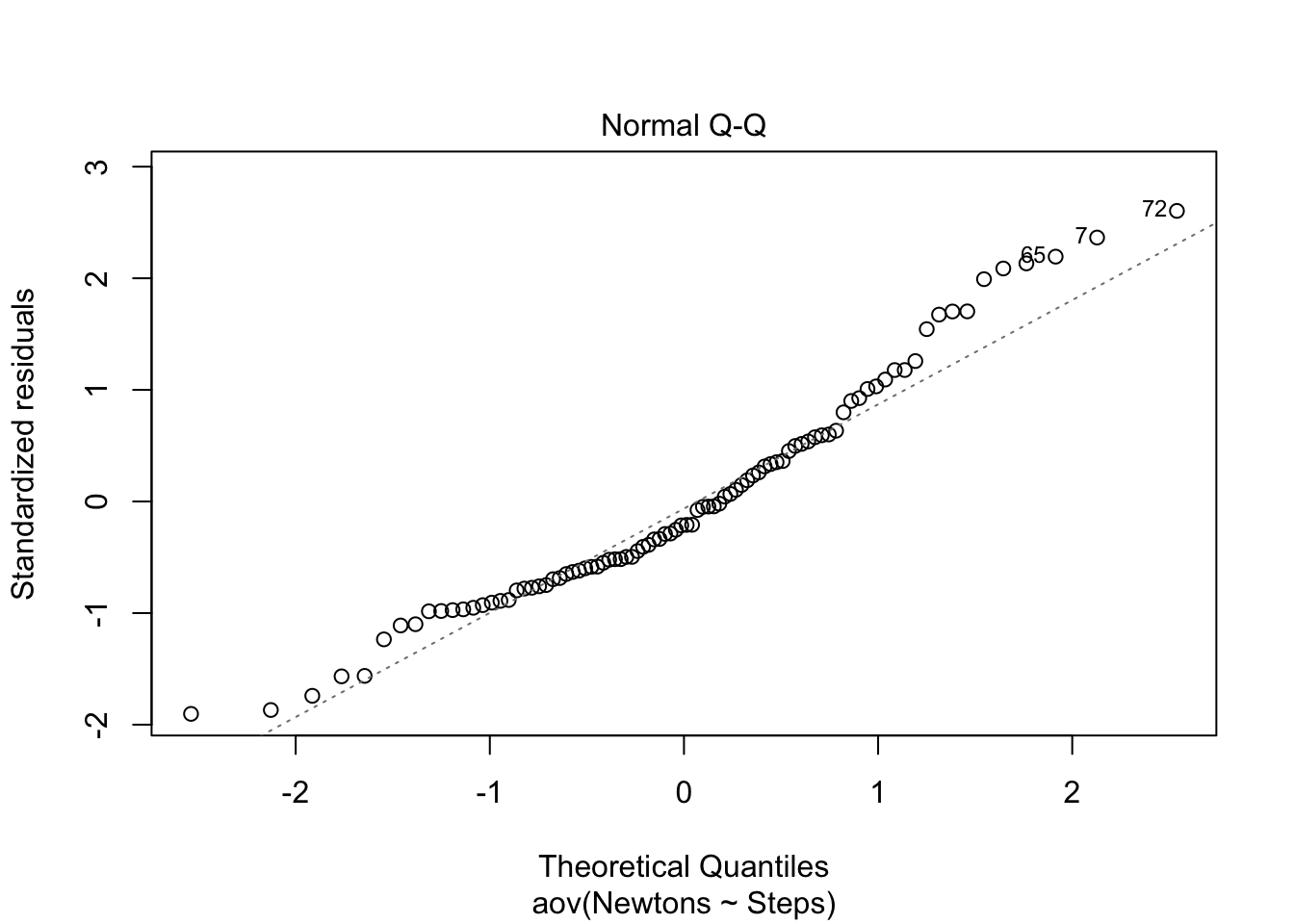

Homogeneity of Variance Test

As in the examination of normality above, base R also can also plot the Residuals vs Fitted values to examine homogeneity of variance. The plot maintains a straight red line which is what would be expected for data that meet the homogeneity of variance assumption. When the assumption of homogeneity of variance is violated one can explore the use of a robust ANOVA.

Code

plot(aov(formula = Newtons ~ Steps, data = WelchANOVA_df), 1)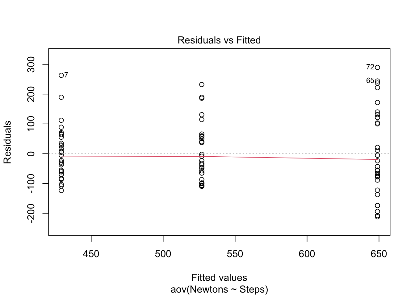

Finally, we can use the rstatix levene_test()(Kassambara 2023) function for the homogeneity of variance test, specifying a formula and a data frame.

Code

levene <- 
  levene_test(formula = Newtons ~ Steps, data = WelchANOVA_df) # significant p-value means the data did not meet the assumption of homogeneity of variance.

gt(levene)

df1	df2	statistic	p
2	87	3.970743	0.02237434

The result is a significant p-value for the test statistic. This indicates that the data does not meet the assumption of homogeneity of variance – we did not meet the assumption of homogeneity of variance (equal variances).

Boxplot

However, if we simply apply the boxplot()(2022b) function, we will visualize the means of each group and can see the variances are not equal, thus violating the assumption of equal mean variances across groups.

Code

# Here we are going to check our assumptions: are the group means variances equal; is the homogeneity of variance assumption violated?

boxPlot1 <- 
  boxplot(Newtons ~ Steps, data = WelchANOVA_df, col = "lightgray")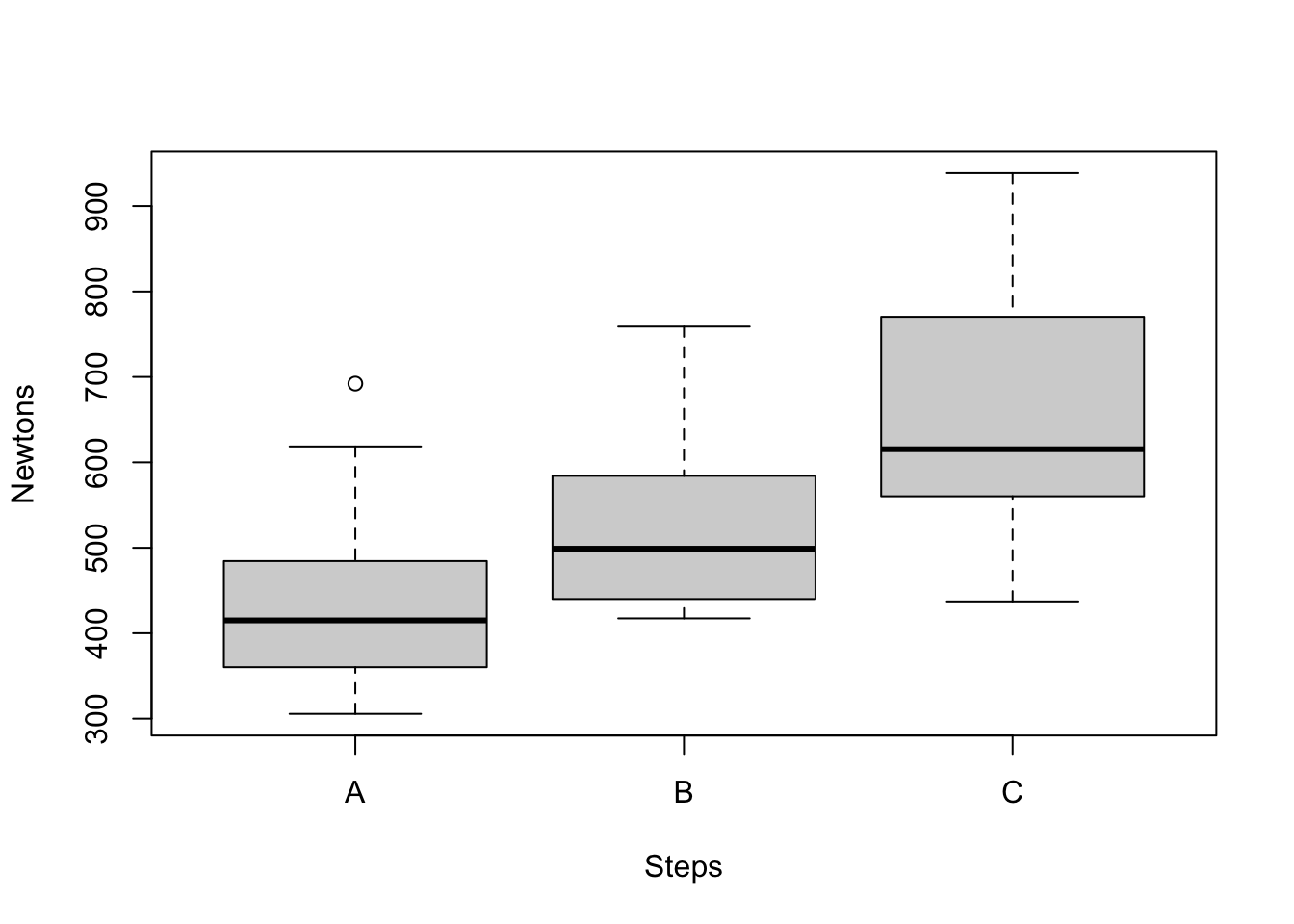

Welch’s ANOVA tests

There are three ways we can conduct the Welch’s ANOVA test:

oneway.test() in the base r(2022a)
welch_anova_test() in the rstatix package(Kassambara 2023)
anovaOnew() in the jmv package(Selker et al. 2022)

We will first describe the first method using the base r function, then describe the second method using the rstatix package, then the last method using the jmv package.

Welch’s ANOVA in `base r`

In base r, we can run the Welch’s ANOVA using the oneway.test() function. We need to provide the formula, the data, and whether we are assuming the mean variances of each group are equal (in this case, we put FALSE)

Code

# Base-R welch anova test
# Analysis of Variance (Welchs) using the base R functions
oneWay <- # naming the test in the global environment
  oneway.test(formula = Newtons ~ Steps, data = WelchANOVA_df, var.equal = FALSE)

oneWay


    One-way analysis of means (not assuming equal variances)

data:  Newtons and Steps
F = 26.19, num df = 2.000, denom df = 56.184, p-value = 9.196e-09

The p-value is in scientific notation, so we ask R if the p-value provided is significant with oneWay$p.value < 0.05and the result is:

[1] TRUE

Our Welch’s ANOVA here shows the test statistic is 26.19, which is significant at the p<0.05 level.

Welch’s ANOVA in the `rstatix package`

In the rstatix package we can run the Welch’s ANOVA using the welch_anova_test() function. Here we will need to input the formula. After we input the formula, we can change the p-value from scientific notation to standard numeric value.

Code

# converting the group variable to a factor
WelchANOVA_df$Steps <- 
  as.factor(WelchANOVA_df$Steps)

# rstatix package Welchs ANOVA
Welch <- 
  WelchANOVA_df %>% 
  welch_anova_test(
    Newtons ~ Steps)  

Welch$p <- 
format(Welch$p, scientific = FALSE) # updating the p-value from scientific notation to standard numeric value

gt(Welch)

.y.	n	statistic	DFn	DFd	p	method
Newtons	90	26.19	2	56.18426	0.0000000092	Welch ANOVA

Code

# Add the comment about what the DFn and DFd means on the output table:

The results are output using the following column names (and what they mean):

.y.: the y variable used in the test.
n: sample count.
statistic: the value of the test statistic.
p: p-value.
method: the statistical test used to compare groups.

In our Welch’s ANOVA using the rstatix package, we find that our test statistic is 29.19, and our significance is at p<0.05.

Post-Hoc tests

The Games-Howell post hoc test(Kassambara 2023) is most like Tukey’s method for Classic ANOVA. Both procedures do the following: - Control the joint error rate for the entire series of comparisons. - Compare all possible pairs of groups within a collection of groups.

The Games-Howell post hoc test, like Welch’s analysis of variance, does not require the groups to have equal standard deviations. Conversely, Tukey’s method does require equal standard deviations.

Using the games_howell_test() function,(Kassambara 2023), we need to inpit the data, formula, the ocnfidence level, and whether to include the details.

Code

# Performing the games howell post hoc test on the anova 
postHoc1 <- # naming the post hoc object
games_howell_test(data = WelchANOVA_df, # data set to use
                  formula = Newtons ~ Steps, # formula
                  conf.level = 0.95, # confidence level of the interval.
                  detailed = TRUE) # logical value. Default is FALSE. If TRUE, a detailed result is shown. TRUE adds the se, statistic, and method in the table. 

# updating the p-value from scientific notation to standard numeric value
postHoc1$p.adj <- 
format(postHoc1$p.adj, scientific = FALSE)

gt(postHoc1)

.y.	group1	group2	n1	n2	estimate	conf.low	conf.high	se	statistic	df	p.adj	p.adj.signif	method
Newtons	A	B	30	30	97.64867	39.73284	155.5645	17.02184	4.056437	57.47413	0.0004410000	***	Games-Howell
Newtons	A	C	30	30	219.74333	144.72971	294.7570	21.93275	7.084474	48.04134	0.0000000162	****	Games-Howell
Newtons	B	C	30	30	122.09467	45.08372	199.1056	22.55573	3.827585	50.81530	0.0010000000	***	Games-Howell

The resulting output provides the following variable information, with what the result means as follows:

.y.: the y (outcome) variable used in the test.
group1,group2: the compared groups in the pairwise tests.
n1,n2: Sample counts.
estimate, conf.low, conf.high: mean difference and its confidence intervals.
statistic: Test statistic (t-value) used to compute the p-value.
df: degrees of freedom calculated using Welch’s correction.
p.adj: adjusted p-value using Tukey’s method.
method: the statistical test used to compare groups.
p.adj.signif: the significance level of p-values.

Here we find that the greatest variance in means was found in group A to group C, which was 220, with a p<0.05 significance.

Welch’s ANOVA in the `jmv package`(Selker et al. 2022)

The jmv package(Selker et al. 2022) is a suite of common statistical methods such as descriptive’s, t-tests, ANOVAs, regression, correlation matrices, proportion tests, contingency tables, and factor analysis.

The jmv package contains a function that will perform all of the above in one command. Using the anovaOnew() function we can set everything up to automatically perform all of the tests above.

Code

# Conduct Welch's ANOVA using the anovaOneW() function
jmvAnova1 <- 
anovaOneW(
  data = WelchANOVA_df,
  formula = Newtons ~ Steps,
  welchs = TRUE, # TRUE (default) or FALSE, perform Welch's one-way ANOVA which does not assume equal variances
  norm = TRUE, # TRUE or FALSE (default), perform Shapiro-Wilk test of normality
  eqv = TRUE, # TRUE or FALSE (default), perform Levene's test for homogeneity of variances
  phMethod = 'gamesHowell') # 'none', 'gamesHowell' or 'tukey', which post-hoc tests to provide; 'none' shows no post-hoc tests, 'gamesHowell' shows Games-Howell post-hoc tests where no equivalence of variances is assumed, and 'tukey' shows Tukey post-hoc tests where equivalence of variances is assumed. 

jmvAnova1


 ONE-WAY ANOVA

 One-Way ANOVA (Welch's)                                  
 ──────────────────────────────────────────────────────── 
              F           df1    df2         p            
 ──────────────────────────────────────────────────────── 
   Newtons    26.19019      2    56.18426    < .0000001   
 ──────────────────────────────────────────────────────── 


 ASSUMPTION CHECKS

 Normality Test (Shapiro-Wilk)         
 ───────────────────────────────────── 
              W            p           
 ───────────────────────────────────── 
   Newtons    0.9598307    0.0071217   
 ───────────────────────────────────── 
   Note. A low p-value suggests a
   violation of the assumption of
   normality


 Homogeneity of Variances Test (Levene's)           
 ────────────────────────────────────────────────── 
              F           df1    df2    p           
 ────────────────────────────────────────────────── 
   Newtons    5.295575      2     87    0.0067567   
 ────────────────────────────────────────────────── 


 POST HOC TESTS

 Games-Howell Post-Hoc Test – Newtons                             
 ──────────────────────────────────────────────────────────────── 
                           A            B            C            
 ──────────────────────────────────────────────────────────────── 
   A    Mean difference            —    -97.64867     -219.7433   
        p-value                    —    0.0004409    < .0000001   
                                                                  
   B    Mean difference                         —     -122.0947   
        p-value                                 —     0.0010220   
                                                                  
   C    Mean difference                                       —   
        p-value                                               —   
 ────────────────────────────────────────────────────────────────

Here we find similar results to the tests performed above.

Example 2

We used a data set from a small cosmetic company trial of a new cream for treating skin blemishes. It measured the effectiveness of the new cream compared to the leading cream on the market and a placebo. Thirty people were put into three groups of 10 at random, although just before the trial began 2 people from the control group and 1 person from the test group for the existing cream dropped out.

Read Data and Explore

Code

# import the trial data
SkinTr <- read_csv("SkinBlemishTrial.csv")

Code

#Check data
str(SkinTr)

spc_tbl_ [27 × 2] (S3: spec_tbl_df/tbl_df/tbl/data.frame)
 $ SkinBlemishes: num [1:27] 50 39 42 45 38 44 40 49 42 41 ...
 $ Treatement   : chr [1:27] "New" "New" "New" "New" ...
 - attr(*, "spec")=
  .. cols(
  ..   SkinBlemishes = col_double(),
  ..   Treatement = col_character()
  .. )
 - attr(*, "problems")=<externalptr>

Code

# Convert Treatment variable into factor
SkinTr$Treatement <- as.factor(SkinTr$Treatement)

# Explore trial data
str(SkinTr)

spc_tbl_ [27 × 2] (S3: spec_tbl_df/tbl_df/tbl/data.frame)
 $ SkinBlemishes: num [1:27] 50 39 42 45 38 44 40 49 42 41 ...
 $ Treatement   : Factor w/ 3 levels "Control","New",..: 2 2 2 2 2 2 2 2 2 2 ...
 - attr(*, "spec")=
  .. cols(
  ..   SkinBlemishes = col_double(),
  ..   Treatement = col_character()
  .. )
 - attr(*, "problems")=<externalptr>

Code

SkinTr %>%
  group_by(Treatement) %>%
  skim()

Data summary
Name	Piped data
Number of rows	27
Number of columns	2
_______________________
Column type frequency:
numeric	1
________________________
Group variables	Treatement

Variable type: numeric

skim_variable	Treatement	complete_rate	mean	sd	p0	p25	p50	p75	p100	hist
SkinBlemishes	Control	1	35.75	16.30	16	22.75	34	46.75	60	▇▂▂▂▅
SkinBlemishes	New	1	43.00	4.03	38	40.25	42	44.75	50	▇▇▅▁▅
SkinBlemishes	Old	1	33.44	9.30	22	27.00	31	40.00	50	▇▇▁▅▂

Check for ANOVA Assumption

As in example 1 above, we use Q-Q plot, box plot and levene test to check for normality and equal variance.

Code

SkinTr %>%
  ggplot(., aes(x = Treatement, y = SkinBlemishes)) +
  geom_boxplot()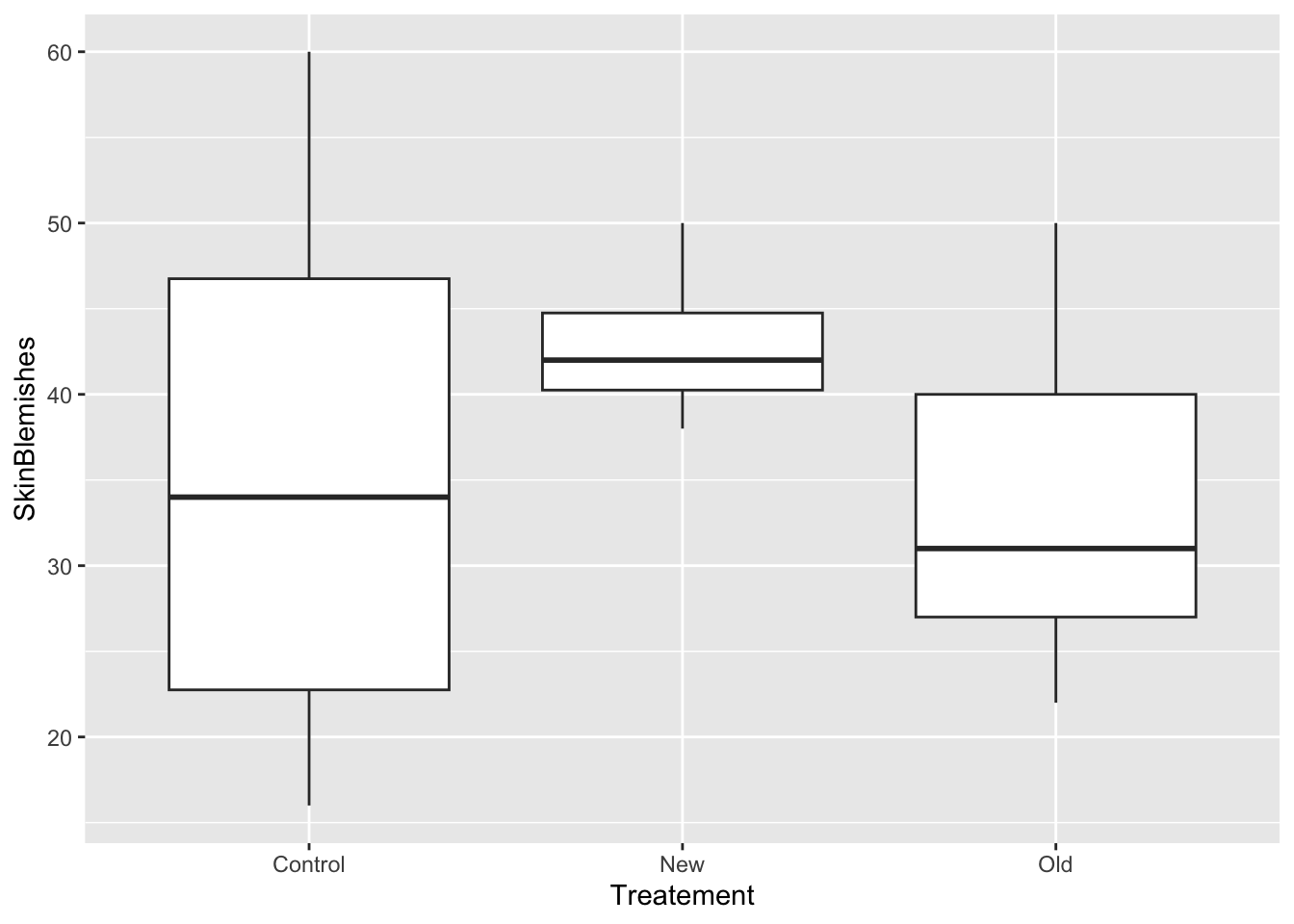

Code

levene2 <- 
  levene_test(data = SkinTr, formula = SkinBlemishes ~ Treatement) 
# significant p-value means the data did not meet the assumption of homogeneity of variance.

gt(levene2)

df1	df2	statistic	p
2	24	6.519442	0.005478229

Since in this data set we can not assume equal variance, we will use Welch’s ANOVA to determine if there is difference between the three skin cream.

Null and Alternative Hypothesis

Null Hypothesis: There is no difference in mean skin blemishes between the three skim cream treatment arms.

Alternative Hypothesis: The three skin cream are not the same.

Welch’s ANOVA Example 2

In this example we use the rstatix package to run the Welch’s ANOVA. You get similar results with other alternatives in explained in example 1.

Code

# running welch's ANOVA
Welch2 <- 
  SkinTr %>% 
  welch_anova_test(
    SkinBlemishes ~ Treatement)  

Welch2$p <- 
format(Welch2$p, scientific = FALSE) 
# updating the p-value from scientific notation to standard numeric value

gt(Welch2)

.y.	n	statistic	DFn	DFd	p	method
SkinBlemishes	27	4.32	2	11.69964	0.039	Welch ANOVA

In this examples, we find that our test statistic is 4.32, and our p value is 0.039. this indicates that there is significant difference between the mean skin blemishes between the three skin cream. To identify which skin cream is different from others we employ post-hoc test.

Post-Hoc Test

We used the Games-Howell post hoc test as in Example 1 above. like Welch’s analysis of variance, does not require the groups to have equal standard deviations. Conversely, Tukey’s method does require equal standard deviations.

Using the games_howell_test() function,(Kassambara 2023), we need to inpit the data, formula, the ocnfidence level, and whether to include the details.

Code

# Performing the games howell post hoc test 
postHoc2 <-
games_howell_test(data = SkinTr, 
                  formula = SkinBlemishes ~ Treatement, 
                  conf.level = 0.95, 
                  detailed = TRUE) # logical value. Default is FALSE. If TRUE, a detailed result is shown. TRUE adds the method in the table. 

# updating the p-value from scientific notation to standard numeric value
postHoc2$p.adj <- 
format(postHoc2$p.adj, scientific = FALSE)

gt(postHoc2)

.y.	group1	group2	n1	n2	estimate	conf.low	conf.high	se	statistic	df	p.adj	p.adj.signif	method
SkinBlemishes	Control	New	8	10	7.250000	-9.758451	24.2584512	4.172983	1.228503	7.686398	0.472	ns	Games-Howell
SkinBlemishes	Control	Old	8	9	-2.305556	-20.016542	15.4054309	4.627070	0.352334	10.844848	0.934	ns	Games-Howell
SkinBlemishes	New	Old	10	9	-9.555556	-18.652223	-0.4588879	2.370276	2.850637	10.657758	0.040	*	Games-Howell

From the Welch’s ANOVA and post-hoc test, we can conclude that there is statistically significant difference in mean skin blemishes between the three skin cream. The observed different is significantly attributed to comparing New cream and Old cream.

Conclusion

In this paper we have explained the Welch’s ANOVA test, the conditions for using it, and three different ways to perform the test in R.

References

Frost, Jim. 2023. “Benefits of Welch’s ANOVA Compared to the Classic One-Way ANOVA.” https://statisticsbyjim.com/anova/welchs-anova-compared-to-classic-one-way-anova/.

Kassambara, Alboukadel. 2023. “Rstatix: Pipe-Friendly Framework for Basic Statistical Tests.” https://CRAN.R-project.org/package=rstatix.

R Core Team. 2022a. “R: A Language and Environment for Statistical Computing.” https://www.R-project.org/.

———. 2022b. “R: A Language and Environment for Statistical Computing.” https://www.R-project.org/.

Selker, Ravi, Jonathon Love, Damian Dropmann, and Victor Moreno. 2022. “Jmv: The ’Jamovi’ Analyses.” https://CRAN.R-project.org/package=jmv.

Introduction

Packages

Data Download

Assumptions

Checking for Normality

Homogeneity of Variance Test

Boxplot

Welch’s ANOVA tests

Welch’s ANOVA in base r

Welch’s ANOVA in the rstatix package

Post-Hoc tests

Welch’s ANOVA in the jmv package(Selker et al. 2022)

Example 2

Read Data and Explore

Check for ANOVA Assumption

Null and Alternative Hypothesis

Welch’s ANOVA Example 2

Post-Hoc Test

Conclusion

References

Welch’s ANOVA in `base r`

Welch’s ANOVA in the `rstatix package`

Welch’s ANOVA in the `jmv package`(Selker et al. 2022)