Code
# First we must install or load the necessary packages
# install.packages("ggpubr")
# install.packages("psych")
# install.packages("tidyverse")

library(ggpubr)
library(psych)
library(tidyverse)
library(skimr)
library(gtsummary)Most parametric tests require that residuals be normally distributed and have equal variance among other assumptions. However, in practice, most data does not fit these assumptions. One approach to dealing with data that violate normality assumption is to transform data (one or more variables) to better follow a normal distribution. In most cases, the dependent variable needs to be transformed however, in complex models and multiples regression, both dependent and independent variables that deviate greatly from normal are transformed.
There is nothing illicit in transforming variables, but care must be exercised on how the results from analyses with transformed variables are reported. For example, when comparing the difference between groups using log-transformed data you would want to present the mean difference. To present means or other summary statistics, you might present the mean of transformed values or back transform means to their original units. Some measurements in nature are naturally normally distributed and does not require prior transformation before analysis. Other measurements are naturally log-normally distributed. These include some natural pollutants in water or air and metabolites in biological systems. In these cases there many low values with fewer high values and even fewer very high values.
Skewness is the measure of symmetry or, more precisely, the lack of symmetry. A distribution or data set is symmetric if the left and right of the centre point look more or less the same.
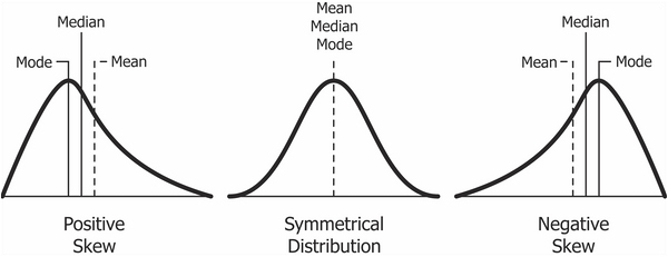
Distribution can be normal, right-skewed (positive skew) or left-skewed (negative skew). For right-skewed data, the tail is on the right, while For left-skewed data the tail is on the left.
common transformation methods include
square root, cube root, and log - For right-skewed data.
square root (constant – x), cube root (constant – x), and log (constant – x) - For left-skewed data.
Another approach is to use a general power transformation, such as Tukey’s Ladder of Powers or a Box-Cox transformation. These methods determine a lambda value, which is used as the power coefficient to transform values. X.new = X ^ lambda for Tukey, and X.new = (X ^ lambda - 1) / lambda for Box-Cox.
Hypothesis - The metobolite data do not meet the assumptions of normality.
To perform a transformation to normality, we need a couple of packages - Some are necessary, and others are preference. We need tidyverse() for reading, wrangling, and visualizing data. We also used ggpubr() for customized visualization of skewness.
ggpubr: ggpubr provides some easy-to-use functions for creating and customizing ‘ggplot2’- based publication ready plots (requires ggplot2)psych- Procedures for Psychological, Psychometric, and Personality Research: A general purpose toolbox developed originally for personality, psychometric theory and experimental psychology.tidyverse: The ‘tidyverse’ is a set of packages that work in harmony because they share common data representations and ‘API’ design.# First we must install or load the necessary packages
# install.packages("ggpubr")
# install.packages("psych")
# install.packages("tidyverse")
library(ggpubr)
library(psych)
library(tidyverse)
library(skimr)
library(gtsummary)As mentioned in the introduction above, some data are naturally log-normally distributed. to demonstrate the transformation of skewed data back to normal, we used a data set that is commonly known to be right skewed. The data set contains urinary metabolites used to predict skeletal muscle wasting associated with cancer. The data can be downloaded from the MetaboAnalyst web page under one-factor statistical examples [data set download]. The original article that published the data can be found Here. Read the data using the read_csv() function.
# Importing the data set from our local drive.
Meta <-
  read_csv("/Users/christoferrodriguez/R_Statistical_Folder/PHC_6099/PHC6900/human_cachexia.csv",
           col_names = TRUE) # Using the column names already assigned in the file.
# We are assigning the data set a name of `Meta` to start so we can explore the
# data. # Display the first 6 rows of the data set
head(Meta) # This shows that there is a lot of columns; we only need three.# A tibble: 6 × 65
`Patient ID` `Muscle loss` `1,6-Anhydro-beta-D-glucose` `1-Methylnicotinamide`
<chr> <chr> <dbl> <dbl>
1 PIF_178 cachexic 40.8 65.4
2 PIF_087 cachexic 62.2 340.
3 PIF_090 cachexic 270. 64.7
4 NETL_005_V1 cachexic 154. 53.0
5 PIF_115 cachexic 22.2 73.7
6 PIF_110 cachexic 213. 31.8
# ℹ 61 more variables: `2-Aminobutyrate` <dbl>, `2-Hydroxyisobutyrate` <dbl>,
# `2-Oxoglutarate` <dbl>, `3-Aminoisobutyrate` <dbl>,
# `3-Hydroxybutyrate` <dbl>, `3-Hydroxyisovalerate` <dbl>,
# `3-Indoxylsulfate` <dbl>, `4-Hydroxyphenylacetate` <dbl>, Acetate <dbl>,
# Acetone <dbl>, Adipate <dbl>, Alanine <dbl>, Asparagine <dbl>,
# Betaine <dbl>, Carnitine <dbl>, Citrate <dbl>, Creatine <dbl>,
# Creatinine <dbl>, Dimethylamine <dbl>, Ethanolamine <dbl>, Formate <dbl>, …We are going to look at the following metabolite variables:
Citrate is involved in both energy production and removal of toxic ammonia. High or Low levels of Citrate can indicate various medical indications that need additional testing. One example of an indication is liver and kidney functioning.
Creatine is an amino acid located mostly in your body’s muscles as well as in the brain. Most people get creatine through seafood and red meat — though at levels far below those found in synthetically made creatine supplements. The body’s liver, pancreas and kidneys also can make about 1 gram of creatine per day.
Creatinine is a chemical waste product of Creatine, which comes from the normal wear and tear of the muscles in the body. Creatinine is filtered out by the kidneys. This test is done to identify the kidney function.
Because we only need these three variables, we will select only the first two columns, plus these three columns and create a new dataset to use in our analysis.
#Create a new data set to use with only our selected columns.
Meta_df <-
  Meta %>%
  select(
    `Patient ID`,
    `Muscle loss`,
    Citrate,
    Creatine,
    Creatinine
  )

# View the first 6 rows of the new data set.
head(Meta_df)
# A tibble: 6 × 5
`Patient ID` `Muscle loss` Citrate Creatine Creatinine
<chr> <chr> <dbl> <dbl> <dbl>
1 PIF_178 cachexic 3714. 196. 16482.
2 PIF_087 cachexic 2618. 213. 15835.
3 PIF_090 cachexic 863. 221. 24588.
4 NETL_005_V1 cachexic 13630. 85.6 20952.
5 PIF_115 cachexic 854. 106. 6768.
6 PIF_110 cachexic 1959. 200. 15678.We are going to explore the data using the describe() function in the psych package. This will provide us with the following information:
# We are going to explore the data by summarizing the data using the describe function in the psych package.
describe(Meta_df)
vars n mean sd median trimmed mad min max
Patient ID* 1 77 39.00 22.37 39.00 39.00 28.17 1.00 77.00
Muscle loss* 2 77 1.39 0.49 1.00 1.37 0.00 1.00 2.00
Citrate 3 77 2235.35 2166.57 1790.05 1928.24 1687.32 59.74 13629.61
Creatine 4 77 126.83 273.22 44.26 71.83 53.88 2.75 1863.11
Creatinine 5 77 8733.97 6477.62 7631.20 7994.69 6621.16 1002.25 33860.35
range skew kurtosis se
Patient ID* 76.00 0.00 -1.25 2.55
Muscle loss* 1.00 0.44 -1.83 0.06
Citrate 13569.87 2.43 9.00 246.90
Creatine 1860.36 4.84 25.42 31.14
Creatinine 32858.10 1.15 1.64 738.19Using the selected metabolites, plot histograms to check for the distribution of specific metabolites. Creatinine, Creatine and Citrate are used as examples but other metabolites can be used. These three metabolites are right skewed (positively skewed).
# Next we will create a histogram to view the data as it currently is.
hist(Meta_df$Citrate,
     main = "Histogram of Citrate",
     xlab = "Citrate")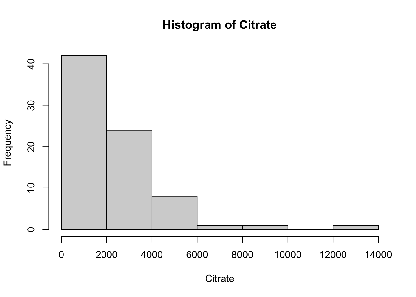
ggplot(data = Meta_df) +
  theme_minimal() +
  aes(sample = Citrate) +
  labs(title = "Citrate levels QQ-plot") +
  stat_qq() + stat_qq_line()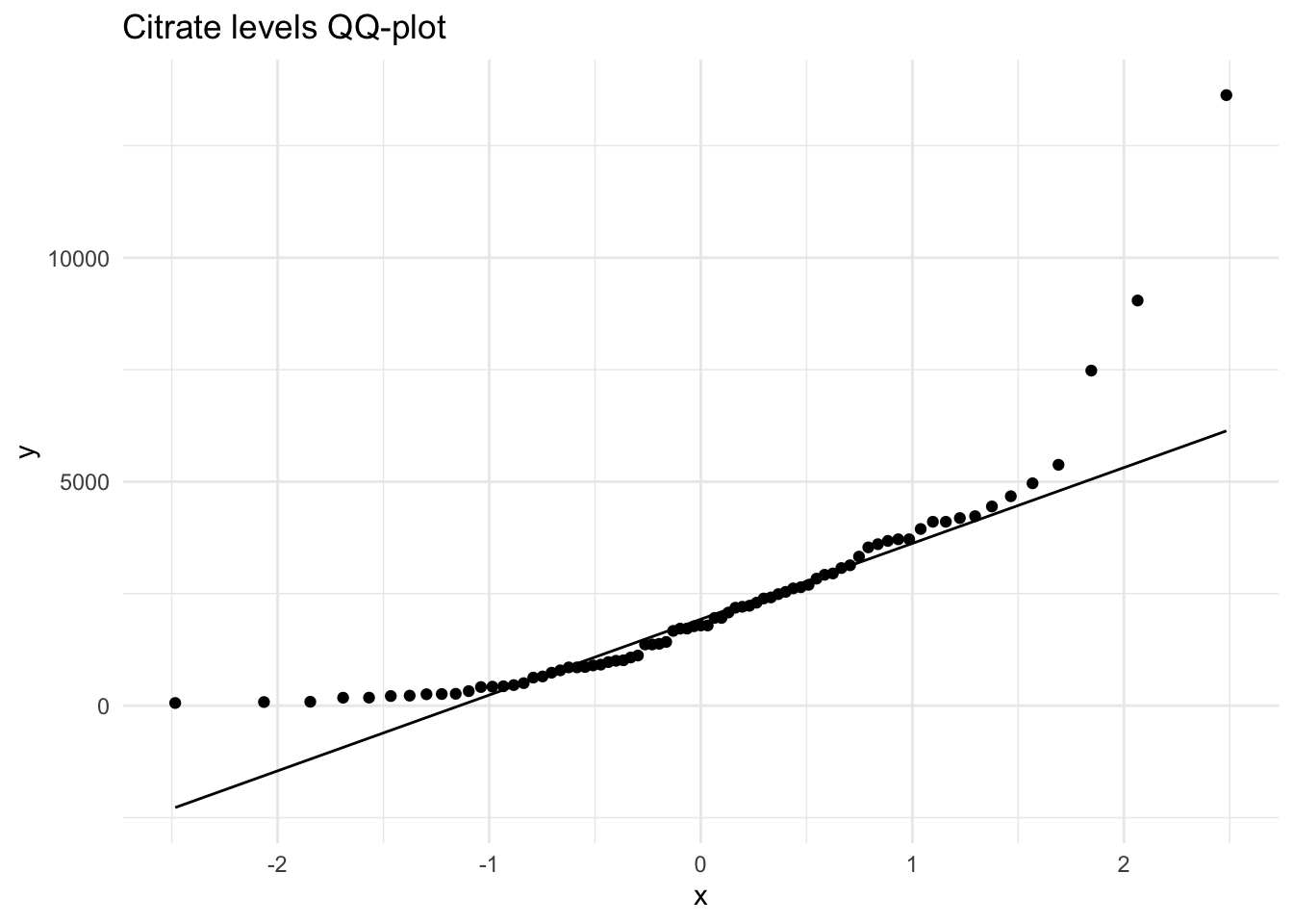
hist(Meta_df$Creatine,
     main = "Histogram of Creatine",
     xlab = "Creatine")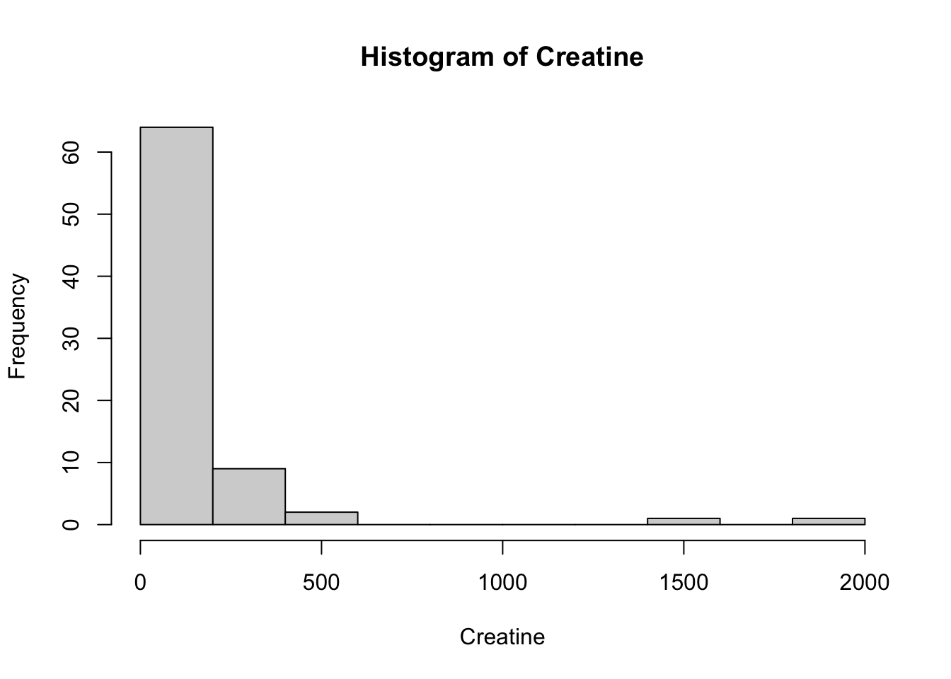
ggplot(data = Meta_df) +
  theme_minimal() +
  aes(sample = Creatine) +
  labs(title = "Creatine levels QQ-plot") +
  stat_qq() + stat_qq_line()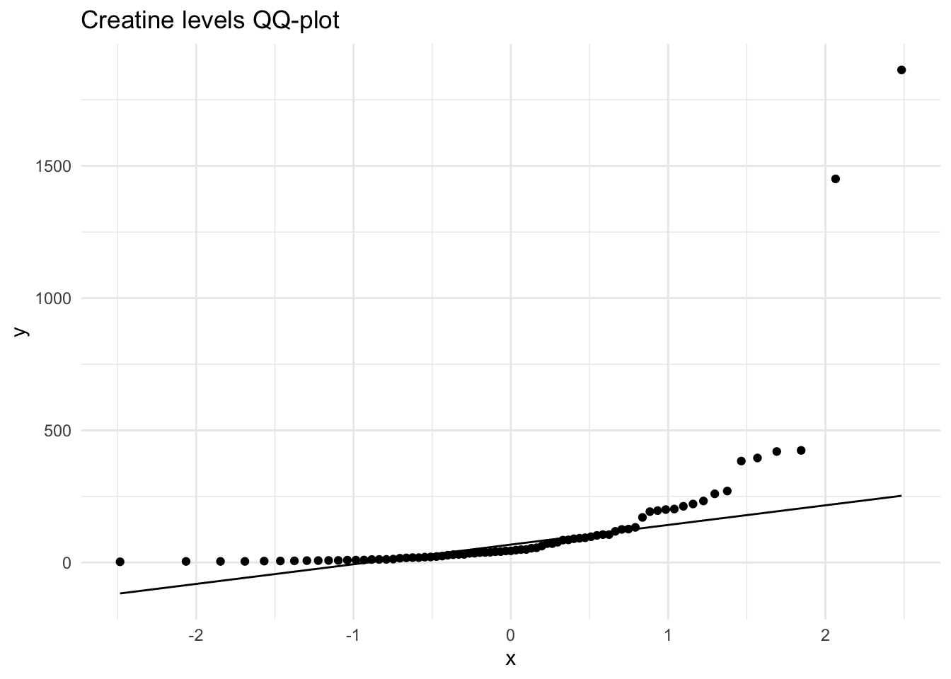
hist(Meta_df$Creatinine,
     main = "Histogram of Creatinine",
     xlab = "Creatinine")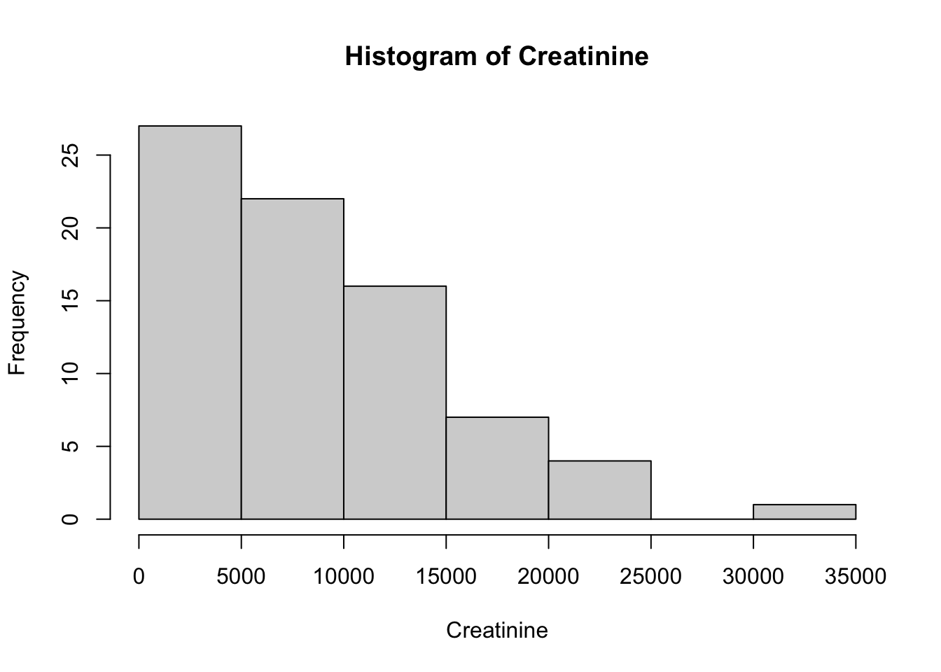
ggplot(data = Meta_df) +
  theme_minimal() +
  aes(sample = Creatinine) +
  labs(title = "Creatinine levels QQ-plot") +
  stat_qq() + stat_qq_line()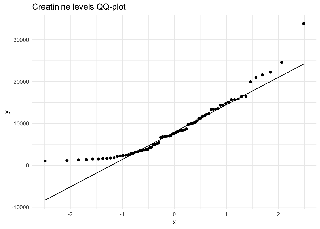
Next, we will create a distribution plot of the current variables to see how it looks compared to a normal distribution plot. To do this, we will use the ggpubr package that will allow us to enhance the ggplot functions available in the tidyverse package. The function we will use is ggdensity.
# Plot the distribution of the Citrate variable
ggdensity(Meta_df$Citrate, fill = "lightgray", title = "Distribution plot of Citrate") +
  scale_x_continuous() +
  xlab("Citrate Level") +
  stat_overlay_normal_density(color = "red", linetype = "dashed")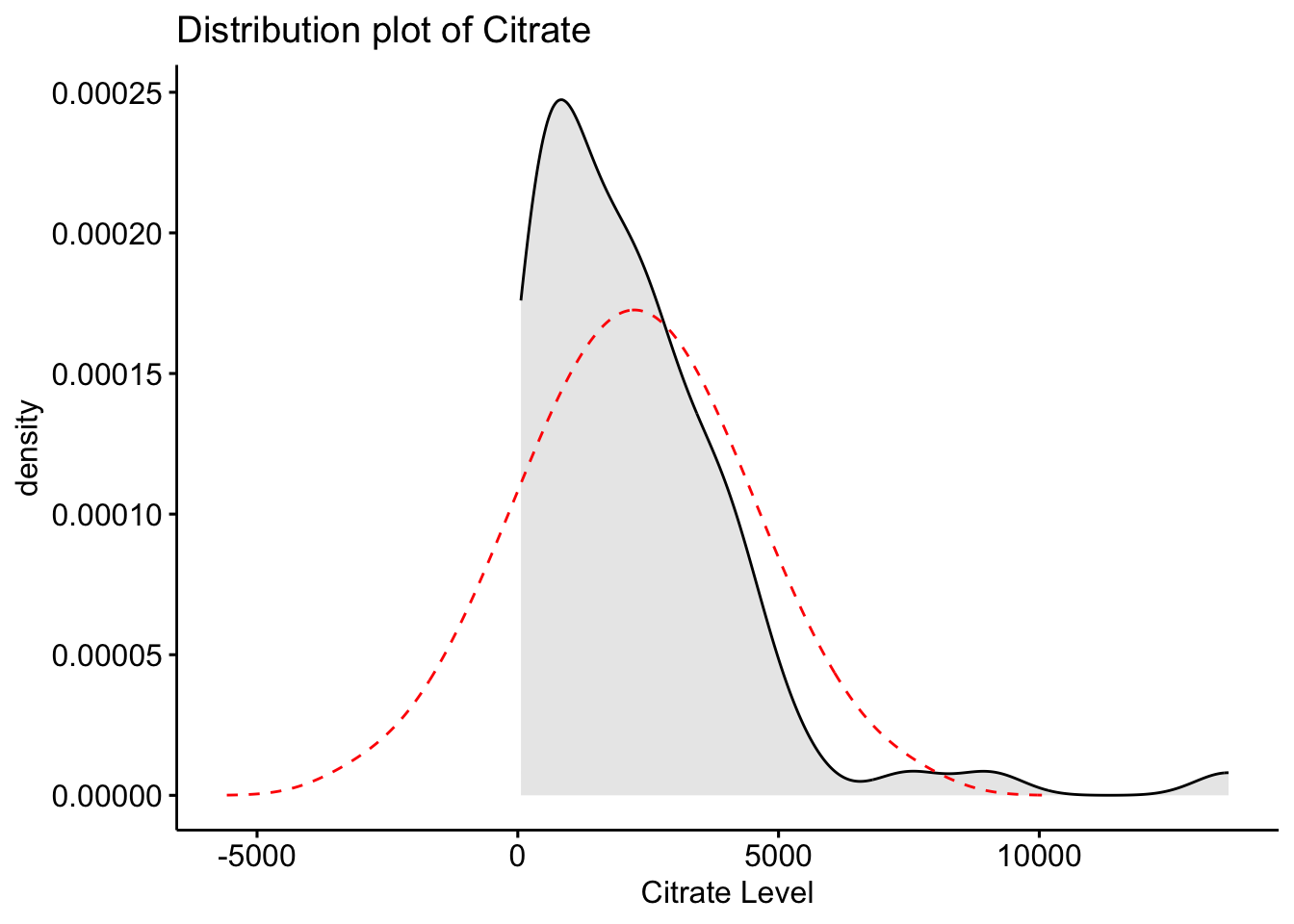
# Plot the distribution of the Creatine variable
ggdensity(Meta_df$Creatine, fill = "lightgray", title = "Distribution plot of Creatine") +
  scale_x_continuous() +
  xlab("Creatine Level") +
  stat_overlay_normal_density(color = "red", linetype = "dashed")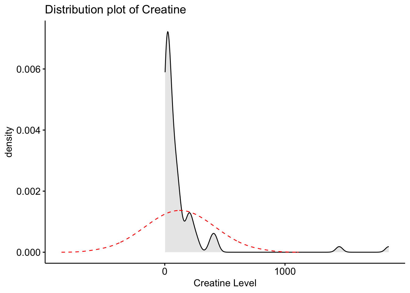
# Plot the distribution of the Creatinine variable
ggdensity(Meta_df$Creatinine, fill = "lightgray", title = "Distribution plot of Creatinine") +
  scale_x_continuous() +
  xlab("Creatinine Level") +
  stat_overlay_normal_density(color = "red", linetype = "dashed")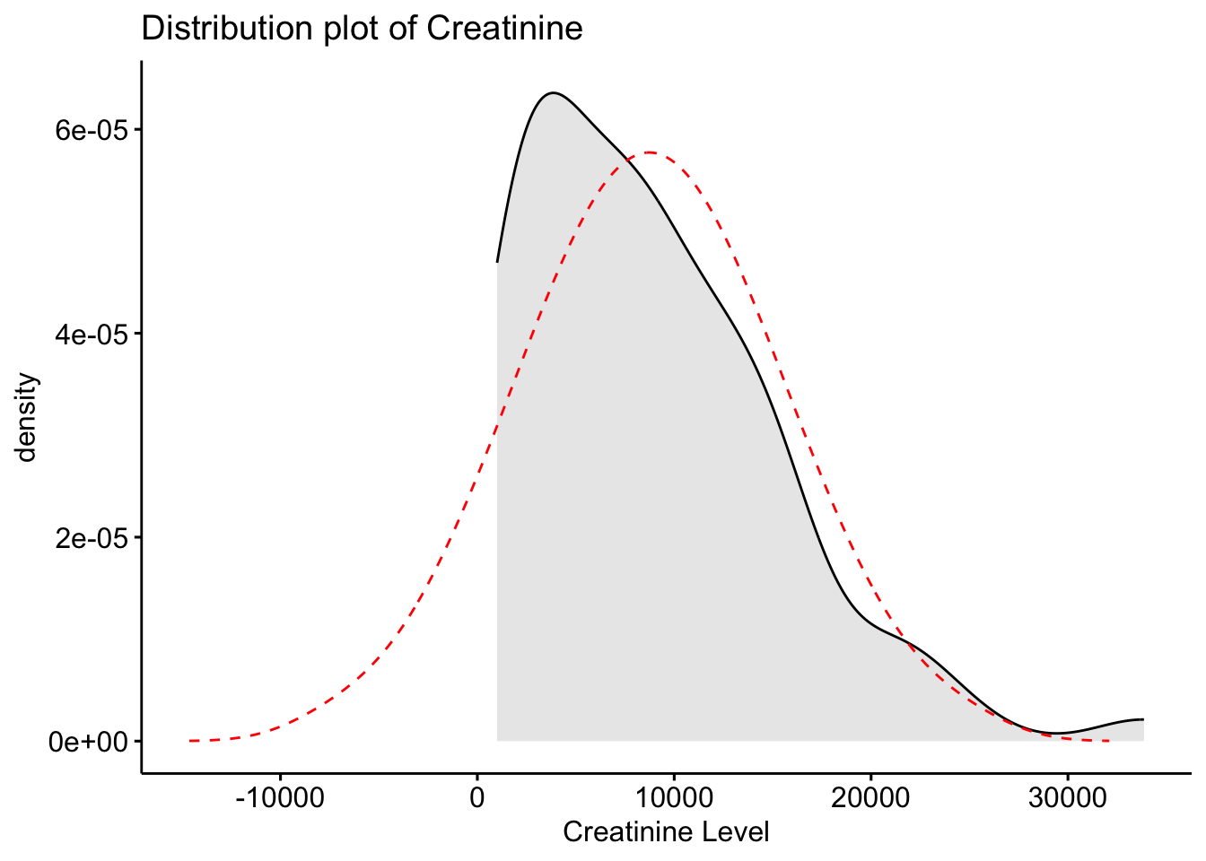
Here we can see that our original variables to not fit the normal distribution, and therefore would need to be transformed.
Now that we see that these variables do not follow the normal distribution, we can identify what type of distribution they are, and what transformation might work best for these variables. To transform right skewed metabolites data, we used square root and log transformation.
# Transforming the original variable into a new rooted variable.
Meta_df$Citrate_root <- sqrt(Meta_df$Citrate)
Meta_df$Creatine_root <- sqrt(Meta_df$Creatine)
Meta_df$Creatinine_root <- sqrt(Meta_df$Creatinine)

# Creating a histogram of the new rooted variables.
hist(Meta_df$Citrate_root,
     main = "Histogram of Citrate (root)",
     xlab = "Citrate (root)")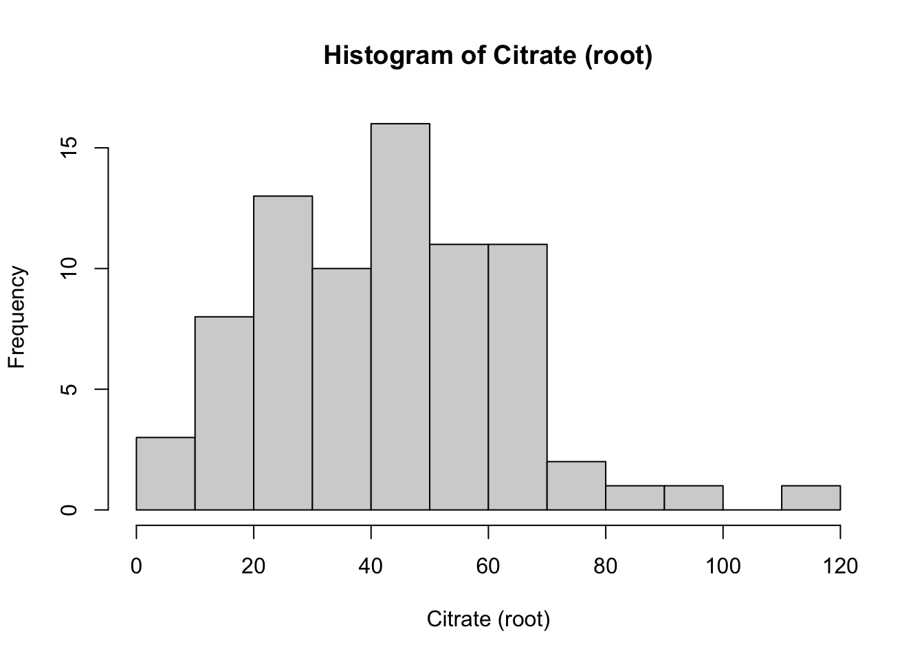
hist(Meta_df$Creatine_root,
     main = "Histogram of Creatine (root)",
     xlab = "Creatine (root)")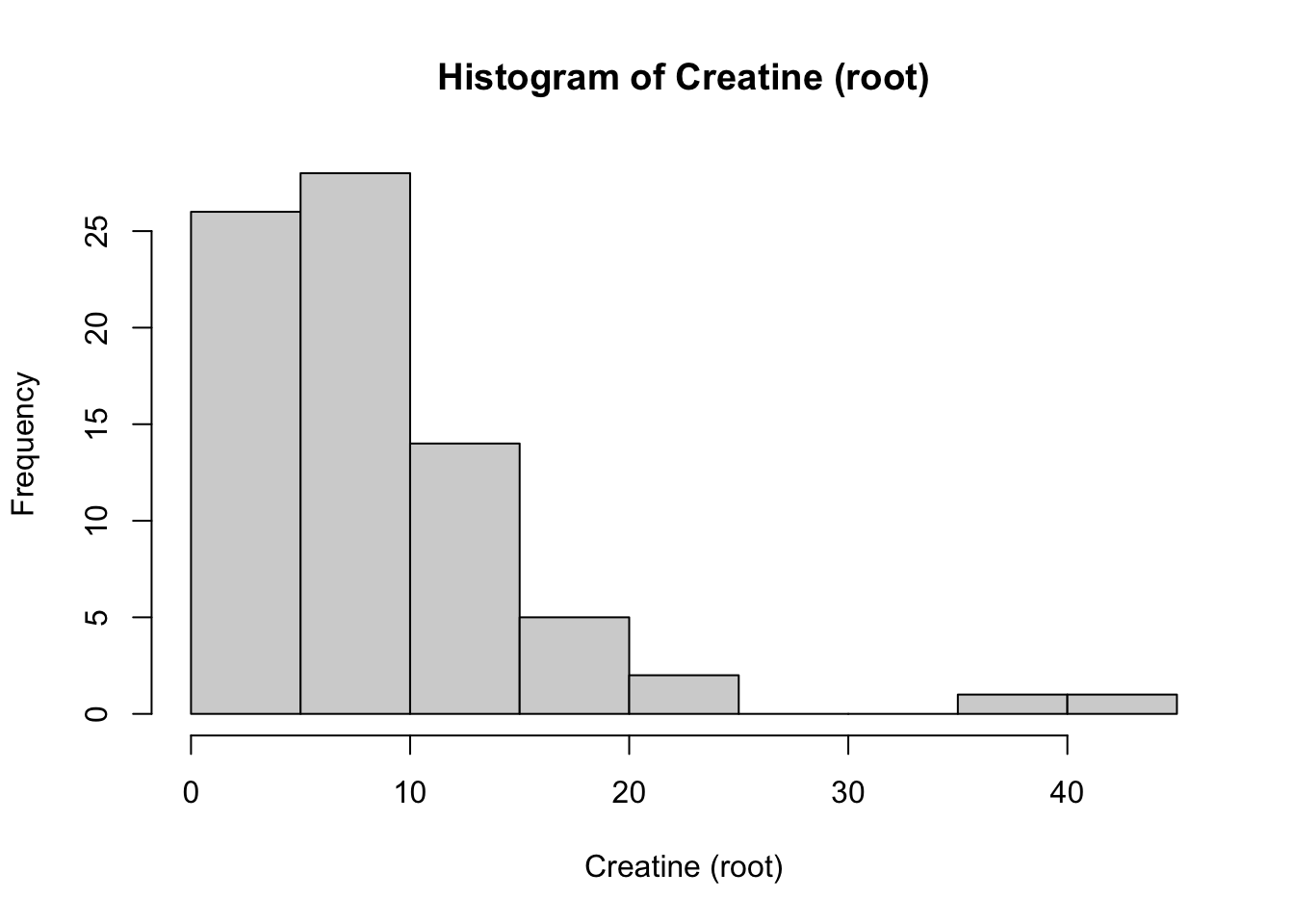
hist(Meta_df$Creatinine_root,
     main = "Histogram of Creatinine (root)",
     xlab = "Creatinine (root)")
# Create a plot of the distribution of the new rooted variable Citrate
ggdensity(Meta_df$Citrate_root, fill = "lightgray", title = "Distribution plot of Citrate (root)") +
  scale_x_continuous() +
  xlab("Citrate (root) Level") +
  stat_overlay_normal_density(color = "red", linetype = "dashed")
# Create a plot of the distribution of the new rooted variable Creatine
ggdensity(Meta_df$Creatine_root, fill = "lightgray", title = "Distribution plot of Creatine (root)") +
  scale_x_continuous() +
  xlab("Creatine (root) Level") +
  stat_overlay_normal_density(color = "red", linetype = "dashed")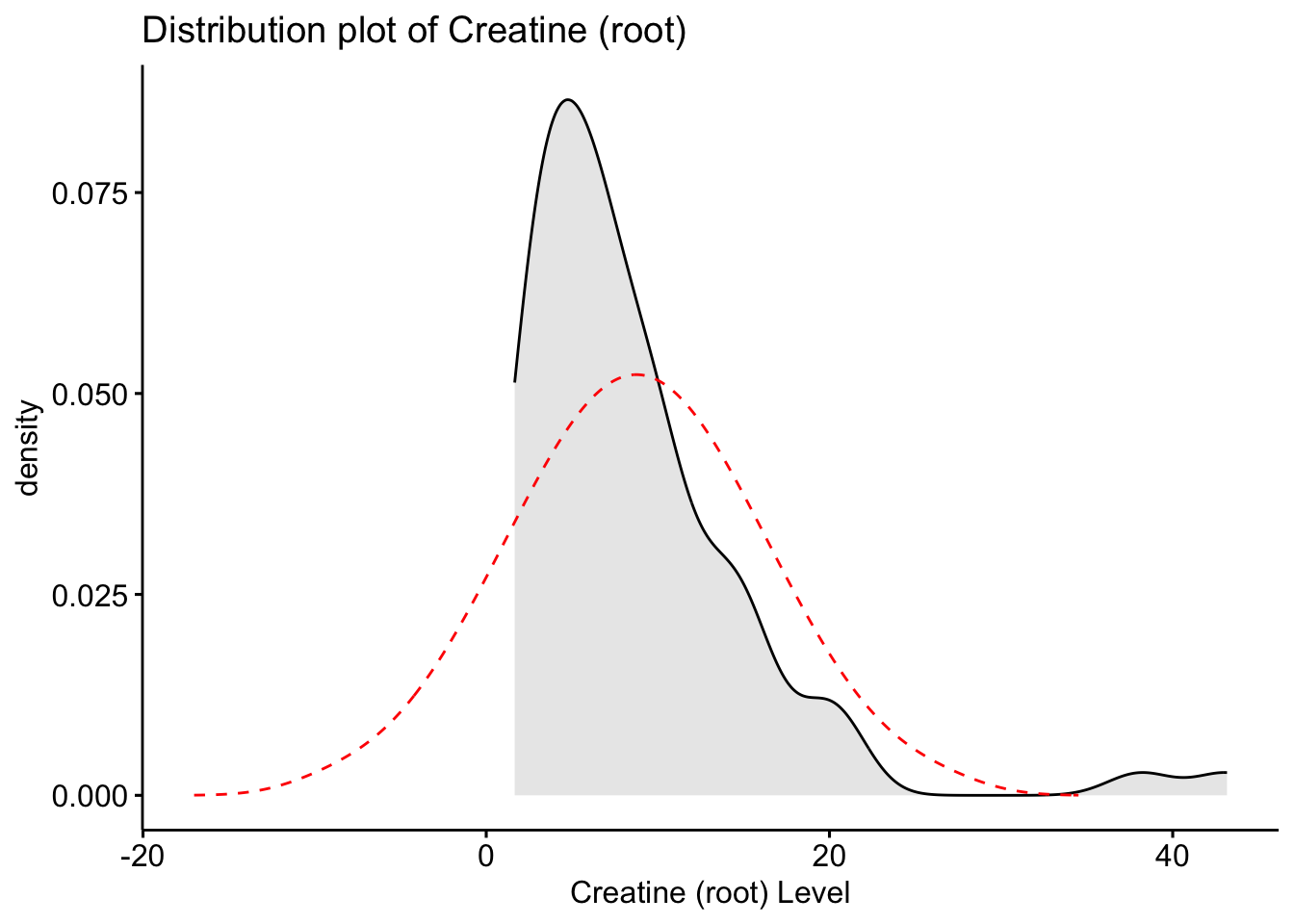
# Create a plot of the distribution of the new rooted variable Creatinine
ggdensity(Meta_df$Creatinine_root, fill = "lightgray", title = "Distribution plot of Creatinine (root)") +
  scale_x_continuous() +
  xlab("Creatinine (root) Level") +
  stat_overlay_normal_density(color = "red", linetype = "dashed")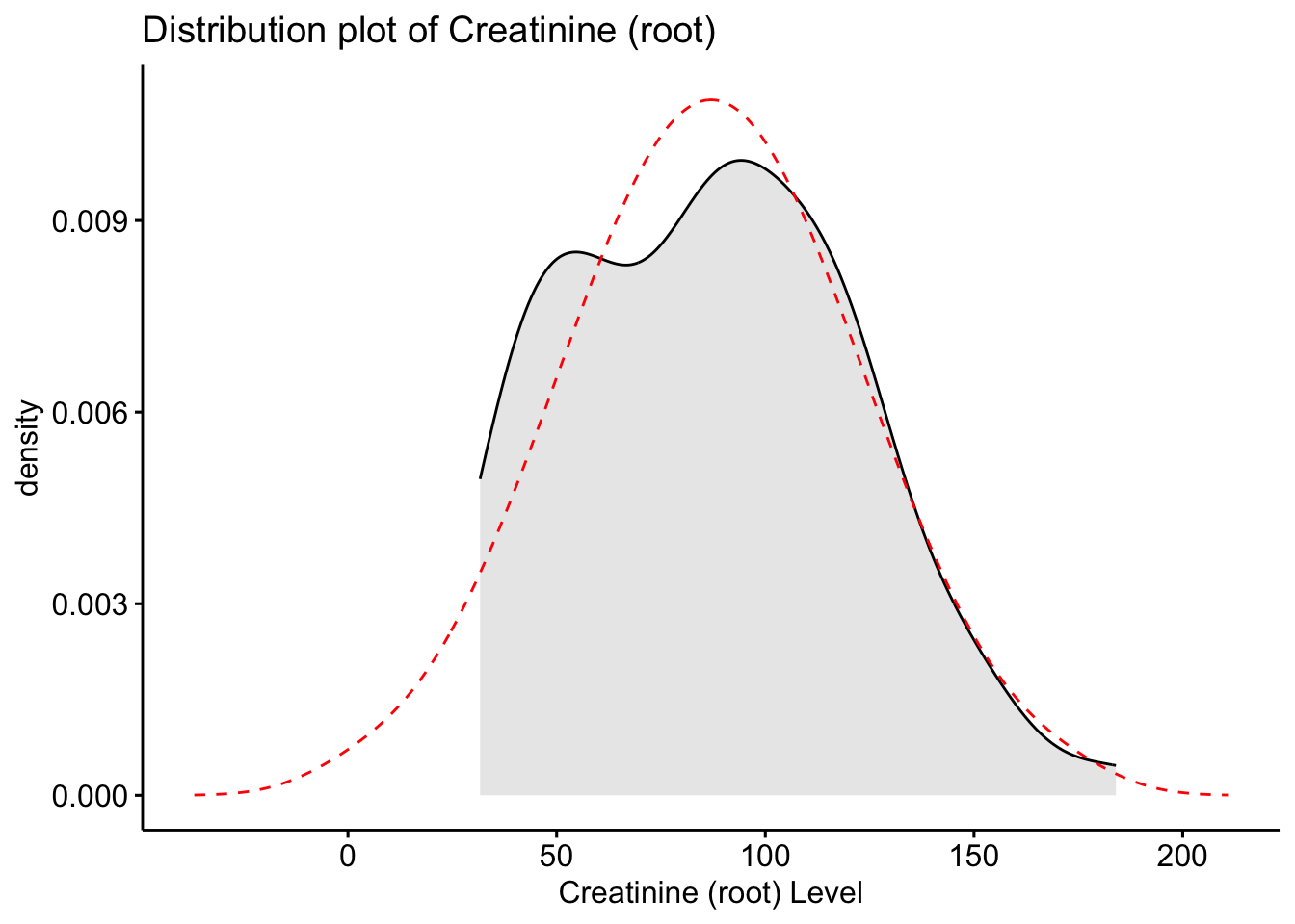
Here we see that the root transformed data is now closer to the normal distribution, however, still is not fully aligned.
# Transforming the original data into a log transformed variable.
Meta_df$Citrate_log <- log(Meta_df$Citrate)
Meta_df$Creatine_log <- log(Meta_df$Creatine)
Meta_df$Creatinine_log <- log(Meta_df$Creatinine)

# Create a histogram and q-q plot of the newly created log transformed variables.
hist(Meta_df$Citrate_log,
     main = "Histogram of Citrate (log)",
     xlab = "Citrate (log)")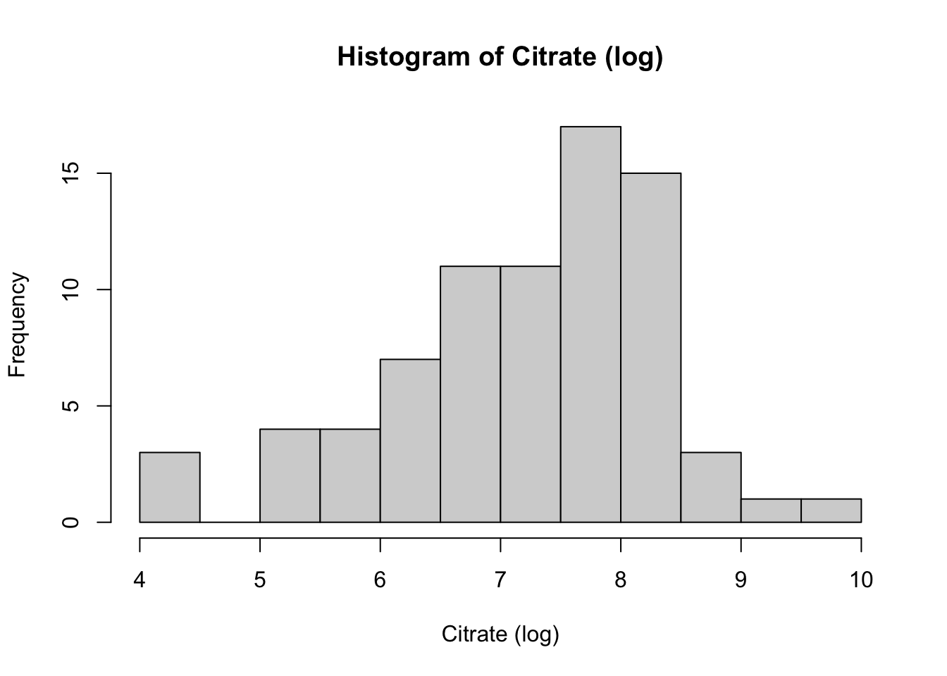
ggplot(data = Meta_df) +
  theme_minimal() +
  aes(sample = Citrate_log) +
  labs(title = "Citrate (log) levels QQ-plot") +
  stat_qq() + stat_qq_line()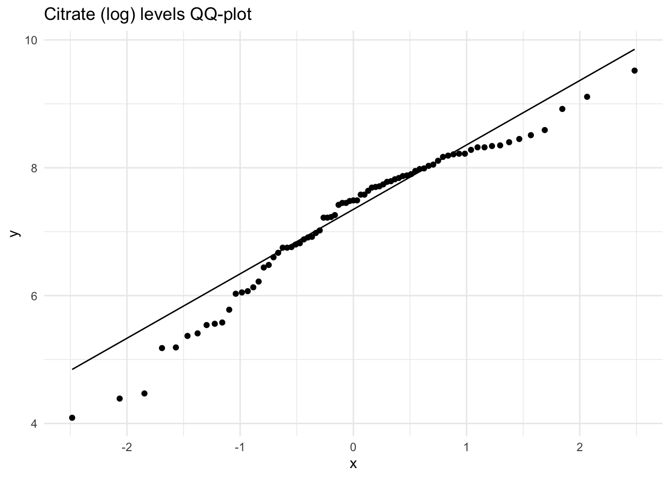
hist(Meta_df$Creatine_log,
     main = "Histogram of Creatine (log)",
     xlab = "Creatine (log)")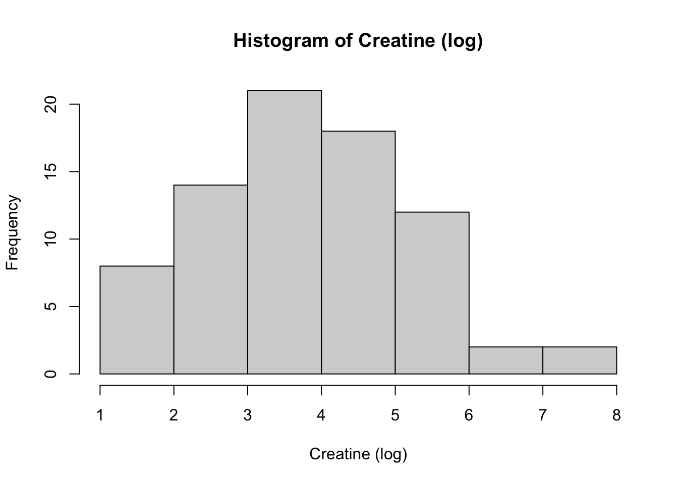
ggplot(data = Meta_df) +
  theme_minimal() +
  aes(sample = Creatine_log) +
  labs(title = "Creatine (log) levels QQ-plot") +
  stat_qq() + stat_qq_line()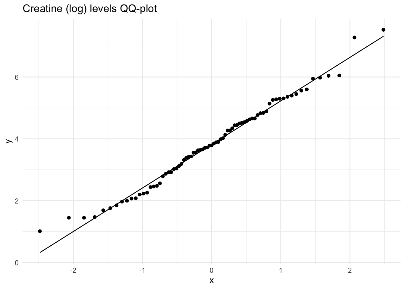
hist(Meta_df$Creatinine_log,
     main = "Histogram of Creatinine (log)",
     xlab = "Creatinine (log)")
ggplot(data = Meta_df) +
  theme_minimal() +
  aes(sample = Creatinine_log) +
  labs(title = "Creatinine (log) levels QQ-plot") +
  stat_qq() + stat_qq_line()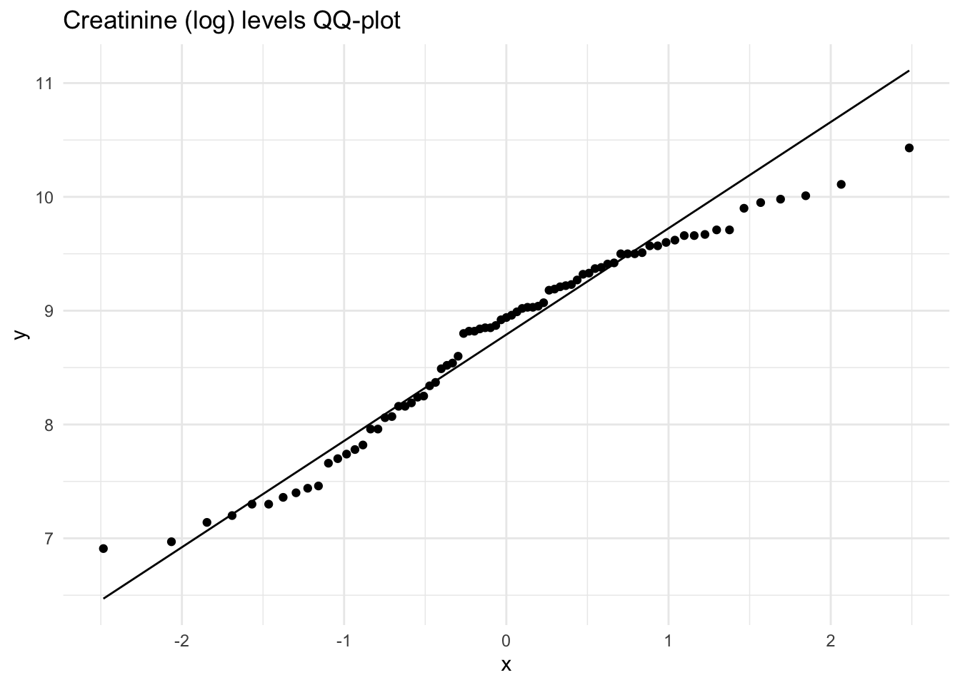
# Create a plot of the distribution of the new log variable for Citrate.
ggdensity(Meta_df$Citrate_log, fill = "lightgray", title = "Distribution plot of Citrate (log)") +
  scale_x_continuous() +
  xlab("Citrate (log) Level") +
  stat_overlay_normal_density(color = "red", linetype = "dashed")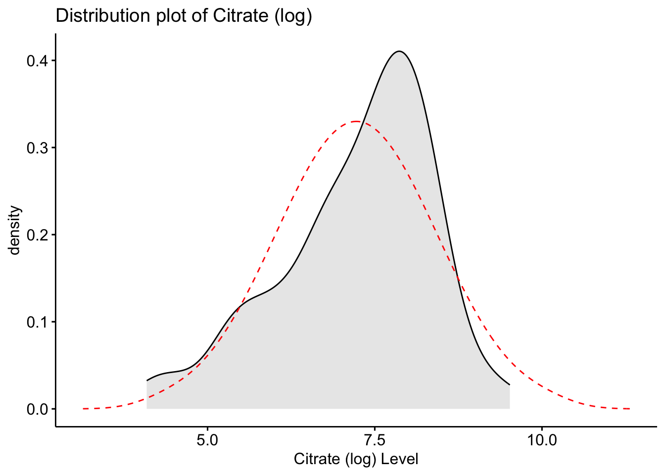
# Create a plot of the distribution of the new log variable for Creatine.
ggdensity(Meta_df$Creatine_log, fill = "lightgray", title = "Distribution plot of Creatine (log)") +
  scale_x_continuous() +
  xlab("Creatine (log) Level") +
  stat_overlay_normal_density(color = "red", linetype = "dashed")
# Create a plot of the distribution of the new log variable for Creatinine.
ggdensity(Meta_df$Creatinine_log, fill = "lightgray", title = "Distribution plot of Creatinine (log)") +
  scale_x_continuous() +
  xlab("Creatinine (log) Level") +
  stat_overlay_normal_density(color = "red", linetype = "dashed")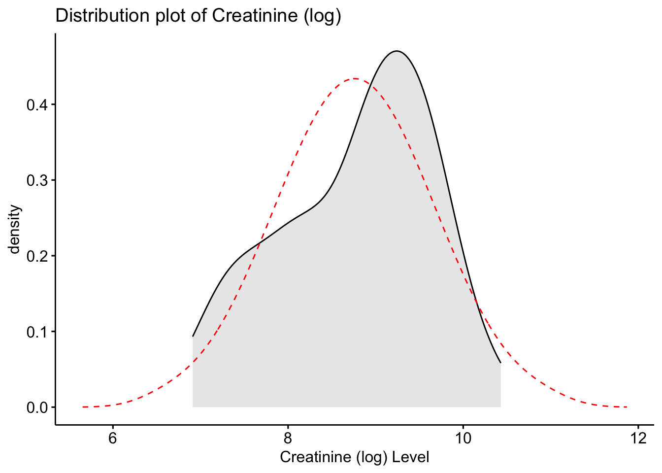
These histograms and plots show that our three variables are now closer to normal distribution, however, two of them might need to be adjusted by using other methods. One thing that can be done is to check the assumptions of normality with these new variables to see if normality has been met. If not, then the data might need to be adjusted accordingly using the other methods of transformation.
Now we will compare the skew and kurtosis values of the new variables.
# Viewing the new skew and kurtosis values for the new rooted and log variables
describe(Meta_df)
vars n mean sd median trimmed mad min
Patient ID* 1 77 39.00 22.37 39.00 39.00 28.17 1.00
Muscle loss* 2 77 1.39 0.49 1.00 1.37 0.00 1.00
Citrate 3 77 2235.35 2166.57 1790.05 1928.24 1687.32 59.74
Creatine 4 77 126.83 273.22 44.26 71.83 53.88 2.75
Creatinine 5 77 8733.97 6477.62 7631.20 7994.69 6621.16 1002.25
Citrate_root 6 77 42.53 20.78 42.31 41.51 20.27 7.73
Creatine_root 7 77 8.74 7.14 6.65 7.62 4.79 1.66
Creatinine_root 8 77 87.01 34.33 87.36 85.64 41.83 31.66
Citrate_log 9 77 7.22 1.13 7.49 7.31 1.04 4.09
Creatine_log 10 77 3.84 1.41 3.79 3.81 1.45 1.01
Creatinine_log 11 77 8.76 0.86 8.94 8.80 0.93 6.91
max range skew kurtosis se
Patient ID* 77.00 76.00 0.00 -1.25 2.55
Muscle loss* 2.00 1.00 0.44 -1.83 0.06
Citrate 13629.61 13569.87 2.43 9.00 246.90
Creatine 1863.11 1860.36 4.84 25.42 31.14
Creatinine 33860.35 32858.10 1.15 1.64 738.19
Citrate_root 116.75 109.02 0.66 0.88 2.37
Creatine_root 43.16 41.51 2.47 8.25 0.81
Creatinine_root 184.01 152.35 0.29 -0.55 3.91
Citrate_log 9.52 5.43 -0.73 0.05 0.13
Creatine_log 7.53 6.52 0.16 -0.42 0.16
Creatinine_log 10.43 3.52 -0.41 -0.84 0.10As you can see, the new rooted variable values for skew and kurtosis are now much lower and than the original variables, with the log transformed variables being the most preferred and acceptable, though additional transformation or testing might be necessary.
describe() function to the skimr() functionskim(Meta_df)| Name | Meta_df |
| Number of rows | 77 |
| Number of columns | 11 |
| _______________________ | |
| Column type frequency: | |
| character | 2 |
| numeric | 9 |
| ________________________ | |
| Group variables | None |
Variable type: character
| skim_variable | n_missing | complete_rate | min | max | empty | n_unique | whitespace |
|---|---|---|---|---|---|---|---|
| Patient ID | 0 | 1 | 7 | 12 | 0 | 77 | 0 |
| Muscle loss | 0 | 1 | 7 | 8 | 0 | 2 | 0 |
Variable type: numeric
| skim_variable | n_missing | complete_rate | mean | sd | p0 | p25 | p50 | p75 | p100 | hist |
|---|---|---|---|---|---|---|---|---|---|---|
| Citrate | 0 | 1 | 2235.35 | 2166.57 | 59.74 | 788.40 | 1790.05 | 3071.74 | 13629.61 | ▇▃▁▁▁ |
| Creatine | 0 | 1 | 126.83 | 273.22 | 2.75 | 17.64 | 44.26 | 117.92 | 1863.11 | ▇▁▁▁▁ |
| Creatinine | 0 | 1 | 8733.97 | 6477.62 | 1002.25 | 3498.19 | 7631.20 | 12332.58 | 33860.35 | ▇▅▂▁▁ |
| Citrate_root | 0 | 1 | 42.53 | 20.78 | 7.73 | 28.08 | 42.31 | 55.42 | 116.75 | ▆▇▆▁▁ |
| Creatine_root | 0 | 1 | 8.74 | 7.14 | 1.66 | 4.20 | 6.65 | 10.86 | 43.16 | ▇▂▁▁▁ |
| Creatinine_root | 0 | 1 | 87.01 | 34.33 | 31.66 | 59.15 | 87.36 | 111.05 | 184.01 | ▇▇▇▃▁ |
| Citrate_log | 0 | 1 | 7.22 | 1.13 | 4.09 | 6.67 | 7.49 | 8.03 | 9.52 | ▁▃▃▇▁ |
| Creatine_log | 0 | 1 | 3.84 | 1.41 | 1.01 | 2.87 | 3.79 | 4.77 | 7.53 | ▃▅▇▃▁ |
| Creatinine_log | 0 | 1 | 8.76 | 0.86 | 6.91 | 8.16 | 8.94 | 9.42 | 10.43 | ▃▃▅▇▂ |
shapiro.test(Meta_df$Citrate_log)
    Shapiro-Wilk normality test

data:  Meta_df$Citrate_log
W = 0.9499, p-value = 0.004245shapiro.test(Meta_df$Creatine_log)
    Shapiro-Wilk normality test

data:  Meta_df$Creatine_log
W = 0.98542, p-value = 0.5266shapiro.test(Meta_df$Creatinine_log)
    Shapiro-Wilk normality test

data:  Meta_df$Creatinine_log
W = 0.95767, p-value = 0.0118Here we found three metabolite variables that were right skewed, and we worked through transforming these variables to meet the assumptions of normal distribution. Now that these distributions have been adjusted, we can use them in analyses like ANOVA or Regression models as long as the normal distribution assumption is not violated.