Generalized Linear Regression - Binary (GLM; Logistic Regression)

Author

Christofer Rodriguez & Said Salehe

Published

June 15, 2023

Introduction

Logistic regression models a relationship between predictor variables and a categorical response variable. For example, you can use logistic regression to model the relationship between exposure to heavy metals in drinking water and development of cancer (a binary variable: either yes or no). Logistic regression helps us estimate a probability of falling into a certain level of the categorical response given a set of predictors. We can choose from three types of logistic regression, depending on the nature of the categorical response variable:

Binary Logistic Regression: Used when the response is binary (i.e., it has two possible outcomes). The Cancer example given above would utilize binary logistic regression. Other examples of binary responses could include passing or failing a test, responding yes or no on a survey, and having high or low blood pressure.

Nominal Logistic Regression: Used when there are three or more categories with no natural ordering to the levels. Examples of nominal responses could include departments at a business (e.g., marketing, sales, HR), type of search engine used (e.g., Google, Yahoo!, MSN), and color (black, red, blue, orange).

Ordinal Logistic Regression: Used when there are three or more categories with a natural ordering to the levels, but the ranking of the levels do not necessarily mean the intervals between them are equal. Examples of ordinal responses could be how students rate the effectiveness of a college course (e.g., good, medium, poor), levels of flavors for hot wings, and medical condition (e.g., good, stable, serious, critical).

For this material we focus more on binary logistic regression.

Why does linear regression not work with binary outcomes?

Binary outcomes only have two values. The example of diabetes disease status, where individuals either have diabetes or they don’t. For our regression model, we could code this outcome so that individuals with diabetes = 1 and those without diabetes = 0. If we just ran a linear regression model with this binary outcome and one continuous predictor variable, then the model will plot a straight line through these points. By visualizing data graphically, it become apparent that linear model does not fit the data well at all when the outcome is binary. The predicted values often correspond to impossible values of the outcome, i.e. values other than 0 or 1. It just doesn’t make sense.

The Logit Link Function

For a binary outcome, we are interested in modelling the proportion of individuals with the outcome of interest. This is equivalent to the probability of an individual having the outcome of interest. Although probabilities are continuous variables, they can only take values from 0 to 1. However, linear models will predict values below 0 and above 1. Luckily, we can transform our variable of interest into one that can be modeled in a regression equation using something called a link function.

As its name suggests, a link function describes the relationship that links our variable of interest to the variable that we use in our regression equation. It’s a mathematical trick. The link function that’s most often used for logistic regression is called the logit. Instead of directly modelling the probability, we model the logit of the probability. The logit of a probability p is equivalent to the natural logarithm (log) of the odds (equation below).

\[ logit (p) = log [\frac{p} {1-p}] = log (Odds) \]

The reason we model the log(odds) rather than just the odds as the outcome variable is because it can take any value from minus infinity (when p = 0) to positive infinity (when p = 1). Odds, on the other hand, can only take positive values. Using the log(odds) as the outcome variable means that we can run a regression model in a similar way to normal linear regression with a continuous variable, and still ensure that the predicted values for probabilities are between 0 and 1.

Assumptions of Logistic Regression

Just as in most regression models, logistic regression has underlying assumptions that needs to be met.

Independence of errors. Using repeated measures or other correlated outcomes the errors will be similarly correlated, and the assumption for errors independence is violated. There are methods for dealing with correlated data using logistic regression techniques, but they are beyond the scope of this material.
Linearity in the logit for any continuous independent variables. There should be a linear relationship between predictor variables and their respective logit-transformed outcomes.
The absence of multicollinearity among independent variables. Example, since weight and body mass index (BMI) are correlated, both should not be included in the same model. A logistic regression model with highly correlated independent variables will usually result in large standard errors for the estimated beta coefficients (or slopes) of these variables. The usual solution is to eliminate one or more redundant variables.

Loading Necessary package

Code

library(gtsummary)
library(tidyverse)

Reading and Tyding Data

We used diabetes data from imperial college of London. The data set has a diabetes variable (dm) for whether someone has diabetes or not (Yes/No). Other variables included in the data set are cholesterol (chol), age, gender (male/female), smoking status (current/never/ex), family history (fh) of diabetes (yes/no), and insurance (non/government/private).

Code

# Read in the leukemia data
DiabetesDF <- read_csv("DiabetesData.csv")

New names:
Rows: 403 Columns: 24
── Column specification
──────────────────────────────────────────────────────── Delimiter: "," chr
(4): location, gender, frame, dm dbl (20): ...1, id, chol, stab.glu, hdl,
ratio, glyhb, age, height, weight, ...
ℹ Use `spec()` to retrieve the full column specification for this data. ℹ
Specify the column types or set `show_col_types = FALSE` to quiet this message.
• `` -> `...1`

Code

# Check imported data and perform necessary transformation
str(DiabetesDF)

spc_tbl_ [403 × 24] (S3: spec_tbl_df/tbl_df/tbl/data.frame)
 $ ...1     : num [1:403] 1 2 3 4 5 6 7 8 9 10 ...
 $ id       : num [1:403] 1000 1001 1002 1003 1005 ...
 $ chol     : num [1:403] 203 165 228 78 249 248 195 227 177 263 ...
 $ stab.glu : num [1:403] 82 97 92 93 90 94 92 75 87 89 ...
 $ hdl      : num [1:403] 56 24 37 12 28 69 41 44 49 40 ...
 $ ratio    : num [1:403] 3.6 6.9 6.2 6.5 8.9 ...
 $ glyhb    : num [1:403] 4.31 4.44 4.64 4.63 7.72 ...
 $ location : chr [1:403] "Buckingham" "Buckingham" "Buckingham" "Buckingham" ...
 $ age      : num [1:403] 46 29 58 67 64 34 30 37 45 55 ...
 $ gender   : chr [1:403] "female" "female" "female" "male" ...
 $ height   : num [1:403] 62 64 61 67 68 71 69 59 69 63 ...
 $ weight   : num [1:403] 121 218 256 119 183 190 191 170 166 202 ...
 $ frame    : chr [1:403] "medium" "large" "large" "large" ...
 $ bp.1s    : num [1:403] 118 112 190 110 138 132 161 NA 160 108 ...
 $ bp.1d    : num [1:403] 59 68 92 50 80 86 112 NA 80 72 ...
 $ bp.2s    : num [1:403] NA NA 185 NA NA NA 161 NA 128 NA ...
 $ bp.2d    : num [1:403] NA NA 92 NA NA NA 112 NA 86 NA ...
 $ waist    : num [1:403] 29 46 49 33 44 36 46 34 34 45 ...
 $ hip      : num [1:403] 38 48 57 38 41 42 49 39 40 50 ...
 $ time.ppn : num [1:403] 720 360 180 480 300 195 720 1020 300 240 ...
 $ insurance: num [1:403] 1 0 2 1 0 1 2 0 2 2 ...
 $ fh       : num [1:403] 0 0 0 0 0 0 1 0 1 0 ...
 $ smoking  : num [1:403] 3 2 2 3 3 1 2 2 1 2 ...
 $ dm       : chr [1:403] "no" "no" "no" "no" ...
 - attr(*, "spec")=
  .. cols(
  ..   ...1 = col_double(),
  ..   id = col_double(),
  ..   chol = col_double(),
  ..   stab.glu = col_double(),
  ..   hdl = col_double(),
  ..   ratio = col_double(),
  ..   glyhb = col_double(),
  ..   location = col_character(),
  ..   age = col_double(),
  ..   gender = col_character(),
  ..   height = col_double(),
  ..   weight = col_double(),
  ..   frame = col_character(),
  ..   bp.1s = col_double(),
  ..   bp.1d = col_double(),
  ..   bp.2s = col_double(),
  ..   bp.2d = col_double(),
  ..   waist = col_double(),
  ..   hip = col_double(),
  ..   time.ppn = col_double(),
  ..   insurance = col_double(),
  ..   fh = col_double(),
  ..   smoking = col_double(),
  ..   dm = col_character()
  .. )
 - attr(*, "problems")=<externalptr>

Code

# Change REMISS into factor variable for binary logistic modelling
DiabetesDF$gender <- as.factor(DiabetesDF$gender)
DiabetesDF$insurance <- as.factor(DiabetesDF$insurance)
DiabetesDF$fh <- as.factor(DiabetesDF$fh)
DiabetesDF$smoking <- as.factor(DiabetesDF$smoking)
DiabetesDF$dm <- as.factor(DiabetesDF$dm)

# Name the levels of factor variables smoking, fh, insurance. 
DiabetesDF$smoking <- 
  recode_factor(DiabetesDF$smoking,  "1" = "Current", "2" = "None", 
                "3" = "Ex")
DiabetesDF$fh <- 
  recode_factor(DiabetesDF$fh, "0" = "No",  "1" = "Yes")

DiabetesDF$insurance <- 
  recode_factor(DiabetesDF$insurance,  "0" = "None",  "1" = "Government",
                "2" = "Private")

Fitting Simple Logistic Regression Model

If we interested in whether cholesterol levels are associated with diabetes, we can fit a simple logistic regression models as follows: Fit1_lr <- glm(dm ~ chol, data = DiabetesDF, family = "binomial")

Code

# Fit Logistic Regression model using GLM
Fit1_lr <- glm(dm ~ chol, data = DiabetesDF, family = "binomial")

Fit1_lr %>% 
  tbl_regression(exponentiate = TRUE) %>% 
  bold_p(0.1)

Characteristic	OR¹	95% CI¹	p-value
chol	1.01	1.01, 1.02	<0.001
¹ OR = Odds Ratio, CI = Confidence Interval

Code

# If you want to get Odds Ratio (OR) use exponentiate = TRUE
# use ?tbl_regression to read the documentation for regression summary table

Here we find that cholesterol is significantly associated with the diagnoses of diabetes.

Fitting Multiple Logistic Regression Model

To adjust for other covariates, we can include multiple variable in our logistic regression model with the following: Fit2_mlr <- glm(dm ~ chol + fh + gender + smoking + insurance, data = DiabetesDF, family = "binomial")

Code

# Fiting Multiple Logistic Regression Model
Fit2_mlr <- glm(dm ~ chol + fh + gender + smoking + insurance, data = DiabetesDF, family = "binomial")

Fit2_mlr %>% 
  tbl_regression(exponentiate = TRUE) %>% 
  bold_p(0.1)

Characteristic	OR¹	95% CI¹	p-value
chol	1.01	1.01, 1.02	<0.001
fh
No	—	—
Yes	2.57	1.33, 4.85	0.004
gender
female	—	—
male	1.17	0.65, 2.08	0.6
smoking
Current	—	—
None	0.80	0.43, 1.54	0.5
Ex	0.88	0.35, 2.11	0.8
insurance
None	—	—
Government	0.75	0.38, 1.49	0.4
Private	0.58	0.28, 1.18	0.14
¹ OR = Odds Ratio, CI = Confidence Interval

After adjusting for other covariates the OR for cholesterol and family history of diabetes are statistically significant.

For a more detailed view of the regression model, use the summary() function to look at the coefficients, the AIC, and other information provided by the model. Or, use $coef at the end to just view the coefficients of each variable.

To calculate Mcfaddens Psuedo $R^2$, we can pull the log-likelihood of the null model out of the logistic variable by getting the value for the null deviance and dividing by -2. Then we can pull the log-likelihood for the model out of the logistic variable by getting the value for the residual deviance and dividing by -2.

Code

# To calculate Mcfaddens Psuedo R2, we can pull the log-likelihood of the null model out of the logistic variable by getting the value for the null deviance and dividing by -2.  Then we can pull the log-likelihood for the model out of the logistic variable by getting the value for the residual deviance and dividing by -2. 

ll.null.1 <- Fit1_lr$null.deviance/-2
ll.proposed.1 <- Fit1_lr$deviance/-2

ll.null.2 <- Fit2_mlr$null.deviance/-2
ll.proposed.2 <- Fit2_mlr$deviance/-2

Then do the math.

Code

(ll.null.1 - ll.proposed.1) / ll.null.1

[1] 0.04459708

Code

(ll.null.2 - ll.proposed.2) / ll.null.2

[1] 0.07427586

Calculate the chi-square values and p-values:

logistic model 1:

Code

# chi-squared
1 - pchisq(2*(ll.proposed.1 - ll.null.1), df=1)

[1] 0.0001122037

Code

1 - pchisq((Fit1_lr$null.deviance - Fit1_lr$deviance), df=1)

[1] 0.0001122037

logistic model 2:

Code

1 - pchisq(2*(ll.proposed.2 - ll.null.2), df=1)

[1] 6.203176e-07

Code

1 - pchisq((Fit2_mlr$null.deviance - Fit2_mlr$deviance), df=1)

[1] 6.203176e-07

Logistic Regression Diagnostics

To check the assumptions, we will look at the data and see if the variables are:

Independence of errors.
Linearity in the logit for any continuous independent variables.
The absence of multicollinearity among independent variables.

Code

# Load the data
DiabetesDF <-
  na.omit(DiabetesDF)

# Fit the logistic regression model
model <- glm(dm ~ chol + fh, DiabetesDF, family = "binomial")

# Predict the probability (p) of diabetes diagnoses
probabilities <- 
  predict(model, type = "response")

predicted.classes <- 
  ifelse(probabilities > 0.5, "Yes", "No")

head(predicted.classes)

   1    2    3    4    5    6 
"No" "No" "No" "No" "No" "No"

Remove qualitative variables from the original data frame and bind the logit values to the data:

Code

# Select only numeric predictors
mydata <- 
  DiabetesDF %>%
  dplyr::select_if(is.numeric) 

predictors <- colnames(mydata)


# Bind the logit and tidying the data for plot
mydata <- 
  mydata %>%
  mutate(
    logit = log(
      probabilities/(1-probabilities)
    )
  ) %>%
  gather(
    key = "predictors", 
    value = "predictor.value", -logit)

Create the scatter plots:

Code

ggplot(
  mydata, 
  aes(
    logit, 
    predictor.value)
  ) +
  geom_point(
    size = 0.5, 
    alpha = 0.5
  ) +
  geom_smooth(
    method = "loess"
  ) + 
  theme_bw() + 
  facet_wrap(
    ~predictors, 
    scales = "free_y"
  )

`geom_smooth()` using formula = 'y ~ x'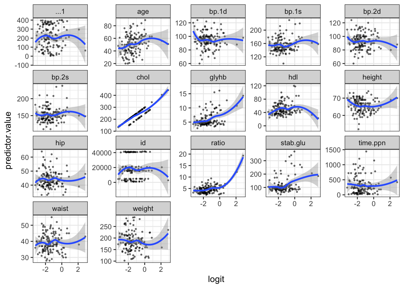

Influential values are extreme individual data points that can alter the quality of the logistic regression model.

The most extreme values in the data can be examined by visualizing the Cook’s distance values. Here we label the top 3 largest values:

Code

plot(model, which = 4, id.n = 3)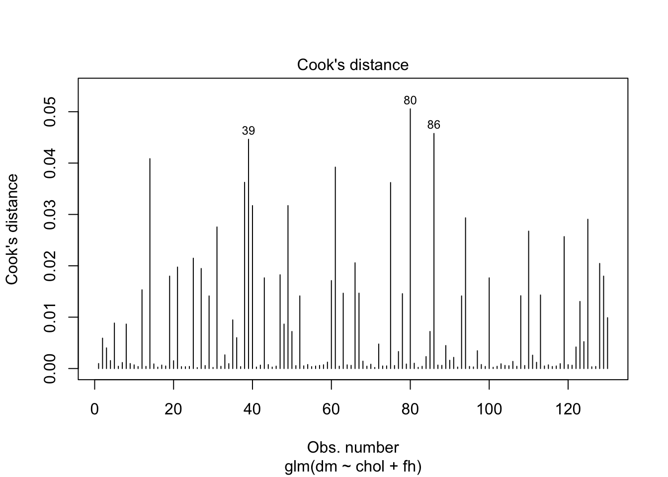

To check whether the data contains potential influential observations, the standardized residual error can be inspected. Data points with an absolute standardized residuals above 3 represent possible outliers and may deserve closer attention.

Code

library(broom)

# Extract model results
model.data <- augment(model) %>% 
  mutate(index = 1:n())

The data for the top 3 largest values, according to the Cook’s distance, can be displayed as follow:

Code

model.data %>% top_n(3, .cooksd)

# A tibble: 3 × 10
  dm     chol fh    .fitted .resid   .hat .sigma .cooksd .std.resid index
  <fct> <dbl> <fct>   <dbl>  <dbl>  <dbl>  <dbl>   <dbl>      <dbl> <int>
1 yes     195 Yes    -1.01    1.63 0.0445  0.963  0.0446       1.66    39
2 yes     173 No     -2.47    2.26 0.0125  0.953  0.0506       2.27    80
3 no      277 Yes     0.613  -1.45 0.0650  0.965  0.0458      -1.50    86

Plot the standardized residuals:

Code

ggplot(model.data, aes(index, .std.resid)) + 
  geom_point(aes(color = dm), alpha = .5) +
  theme_bw()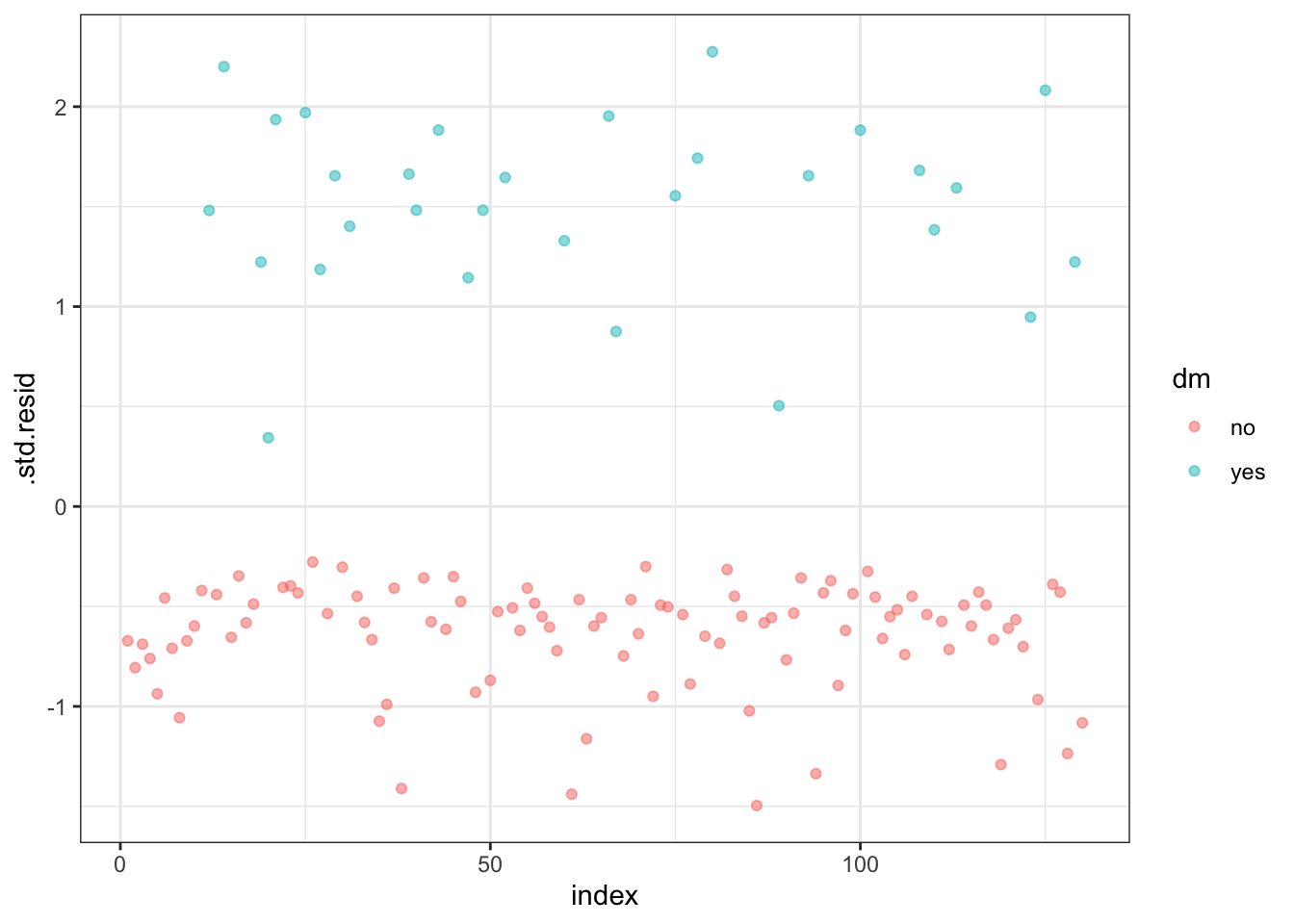

Filter potential influential data points with abs(.std.res) > 2:

Code

model.data %>% 
  filter(abs(.std.resid) > 2)

# A tibble: 3 × 10
  dm     chol fh    .fitted .resid   .hat .sigma .cooksd .std.resid index
  <fct> <dbl> <fct>   <dbl>  <dbl>  <dbl>  <dbl>   <dbl>      <dbl> <int>
1 yes     182 No      -2.30   2.19 0.0120  0.954  0.0409       2.20    14
2 yes     173 No      -2.47   2.26 0.0125  0.953  0.0506       2.27    80
3 yes     196 No      -2.02   2.07 0.0113  0.956  0.0291       2.08   125

When you have outliers in a continuous predictor, potential solutions include:

Removing the concerned records
Transform the data into log scale
Use non parametric methods

Multicollinearity

Multicollinearity is an important issue in regression analysis and should be fixed by removing the concerned variables. It can be assessed using the R function vif() (found in the car package), which computes the variance inflation factors:

Code

car::vif(model)

    chol       fh 
1.007743 1.007743

As a rule of thumb, a VIF value that exceeds 5 or 10 indicates a problematic amount of collinearity. In our example, there is no collinearity: all variables have a value of VIF well below 5.

Conclusion

Here we have described how what a logistic regression is, what the assumptions are for the analysis, and how to perform a logistic regression analysis in R using the glm() function.